w <- c(Rock = 3.2, Jazz = 1.1, Pop = 2.2, EDM = .5)


exp(w) / sum(exp(w))
Rock Jazz Pop EDM
0.64203752 0.07862162 0.23619240 0.04314846
(Modified on 2026-08-12)
261 words
Many research projects involve categorical dependent (or predicted) variables. This means that our data-analysis models output categories or “classes,” rather than continuous numbers. We call this classification: selecting the appropriate output class, given input (independent) variables.
Essentially all categorization models actually do generate numeric output “weights,” which are converted to output categories. In the context of inferential modeling, we postulate that these numeric values represent “latent” variables, which may or may not correspond to actual constructs we are interested in. For example, in logistic regression, any latent value greater than 0 becomes “TRUE”, and vice versa.
\[ \frac{e^{\hat{y}}}{e^{\hat{y}} + 1} > .5 = True \]
For multinomial variables (more than two categories), we typically use the softmax function, which takes a set of weights and (essentially) transforms them to a set of probabilities. For each of \(K\) variables:
\(\frac{e^{x_k}}{\sum^K_{j=1} e^{x_j}}\)
For example, if my model outputs weights \({Rock = 3.2, Jazz = 1.1, Pop = 2.2, EDM = .5}\), softmax results in:
w <- c(Rock = 3.2, Jazz = 1.1, Pop = 2.2, EDM = .5)
exp(w) / sum(exp(w)) Rock Jazz Pop EDM
0.64203752 0.07862162 0.23619240 0.04314846 In statistics, logistic- or multinomial- model parameters are evaluated using maximum likelihood (e.g., cross entropy). There is no “analytical solution” though; algorithms must search for the ML estimate. We then use log-likelihood ratio tests, based on the \(\chi^2\) distribution, to test the significance (\(p < .05\)) of various variables.
Maximimum likelihood and significance tests don’t necessarily tell us how effective a classifier is in an applied setting. We often want more interpretable metrics for classification performance. Binary classification is the most basic case, and many terminologies and methodologies relate to binary classification. A particularly fundamental case is a binary variable corresponding to True and False:
| Positive | Negative | |
|---|---|---|
| True | True positive | False negative (Type 2 error) |
| False | False positive (Type 1 error) | True negative |
However, there are other binary variables, for example Left and Right:
| Predicted Left | Predicted Right | |
|---|---|---|
| Actual Left | True | False |
| Actual Right | False | True |
The binary confusion matrix has four values and provides the complete picture of classification accuracy. However, we often want to reduce this to a single, “overall” metric. Unfortunately, many different metrics are used to quantify aspects of classification error: sensitivity, specificity, precision, negative predictive value, fall-out, false discovery rate, positive likelihood ratio, etc. Often, different names are used for the same things in different fields. I highly recommend wikipedia’s detailed coverage.
Why do we need all these metrics? What’s wrong with the obvious choice, accuracy?
\(\frac{True}{Total}\)
The problem with accuracy is most obvious when you have unbalanced data. For example, I once worked on a project where we tried to predict which notes in a corpus of chorale music were “non-chord tones.” Unfortunately, in the 371 chorales by J.S. Bach, about 92.3% of the 169,050 notes are chord-tones. If our classifier simply guessed that all notes are chord tones…
| Predicted Non-Chord Tone | Predicted Chord Tone | |
|---|---|---|
| Actual Non-Chord Tone | 0 | 13,071 |
| Actual Chord Tone | 0 | 156,033 |
It would get 92.3% accuracy!
The fundamental issue here, is that the rates of Type 1 (false positive) and Type 2 (false negative) errors are always linked. In this chorale example, by always guessing “chord tone,” we made 0 Type 1 errors. All of our 13,071 errors (8.7% of total) were Type 2 errors (false negatives). A classifier can always trade-off between false negatives/positives.
This chorale-music example might seem like a dumb case, but we can do it in any logistic regression by changing the threshold we use. If we set the activation threshold to \(p = .5\) (the usual assumption) we get:
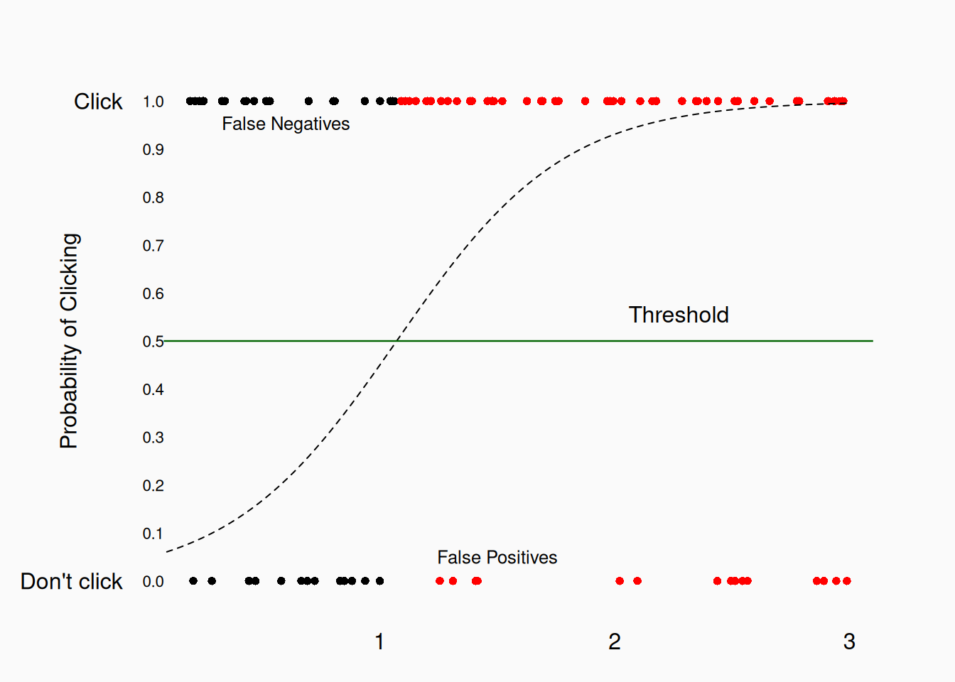
If we raise that threshold to \(p = .7\)…
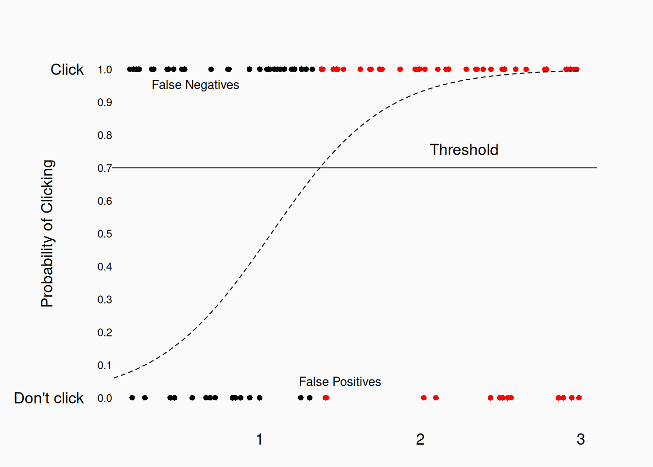
…fewer false positives, but more false negatives. We can always do this. This is why researchers in various fields have developed different metrics and approaches to balancing between false positives and false negatives. The different approaches represent different priorities in different fields. In medicine, false negatives can be life-threatening, but false-positives can potentially waste billions of dollars. The main metrics used in medicine are sensitivity and the specificity, specifically aimed at trade-offs in this domain.
In Machine Learning, the most common classification metrics are precision, recall and the \(F_1\)-score.
In my chorale-music example…
| Predicted Non-Chord Tone | Predicted Chord Tone | |
|---|---|---|
| Actual Non-Chord Tone | 0 | 13,071 |
| Actual Chord Tone | 0 | 156,033 |
See how these metrics tell us more about how well our classifier works (bad) than just the accuracy?
In our comparison of two logistic regressions with two cutoffs (.5 or .7)…
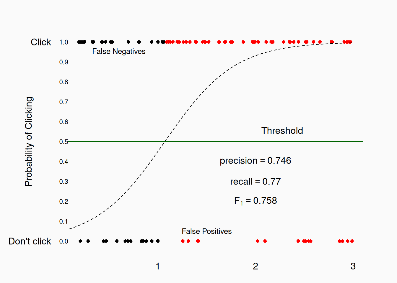
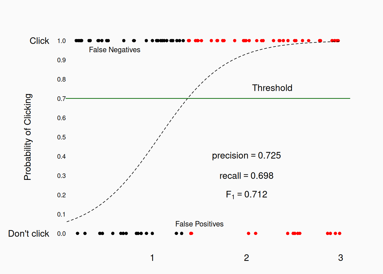
The metrics change subtly, because the underlying classifier is the same. Nonetheless, we see that raising the threshold has a bigger impact on recall (in this case).
Another approach is based on the Receiver Operating Characteristic (ROC), a metric developed during WWII to guide the decisions of radar operators. To create an ROC curve, you plot the true positive rate vs the false positive rate for every possible threshold. The result looks like this:
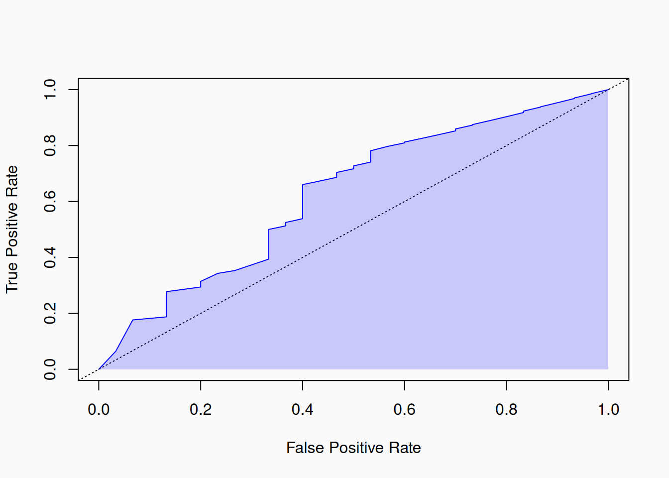
The Area Under the Curve (AUC) is often used as a metric. It ranges from 0.5 (random chance) to 1 (perfect classification). The score is averaged across all thresholds, so it is more abstract.
When we have more than two levels, there is no easy/obvious way to reduce the confusion matrix to a single number. Here is an example predicting “Favorite Genre” from our Describing Data assignment.
# weights:  455 (384 variable)
initial  value 11675.460894
iter  10 value 10314.461455
iter  20 value 9482.118181
iter  30 value 9049.907118
iter  40 value 8798.142573
iter  50 value 8584.351547
iter  60 value 8394.859098
iter  70 value 8279.939109
iter  80 value 8106.650742
iter  90 value 8006.168105
iter 100 value 7895.335068
final  value 7895.335068
stopped after 100 iterations
            Classical Country  EDM Jazz  Pop  Rap Rock
  Classical         0       2    0    2    2    7  287
  Country           1    1154   12    1    2   71  139
  EDM               1     243   71   10    0   42  413
  Jazz              0      64    0   55    0    0    1
  Pop               0     177    2    1  148   76  256
  Rap               1     326   16   10   49  383  175
  Rock              1     144    4    9   21   23 1598
Notice that the data is highly unbalanced: Country and Rock are by far the most common favorite genre, and the model accordingly guesses them a lot.
The accuracy is 56.8% Is that good? To answer that, we have to think about what the baseline is here. You might think that since there are six categories, the baseline (null hypothesis) guessing rate would be \(\frac{1}{6} = 16.\bar{6}\)%. This assumes that a “null model” would just guess randomly (equally) between all six categories. However, our data is unbalanced. Rock music makes up 30% of the favorite genres, so a “null model” would actually guess Rock every time, getting an accuracy of 30%!
For a multinomial classifier, there is no way to calculate “overall” precision/recall etc. The common approach is to calculate precision/recall/F1 for each category independently.
            Classical Country  EDM Jazz  Pop  Rap Rock
  Classical         0       2    0    2    2    7  287
  Country           1    1154   12    1    2   71  139
  EDM               1     243   71   10    0   42  413
  Jazz              0      64    0   55    0    0    1
  Pop               0     177    2    1  148   76  256
  Rap               1     326   16   10   49  383  175
  Rock              1     144    4    9   21   23 1598
Genre Precision Recall F1
<char> <num> <num> <num>
1: Classical 0.000 0.000 NaN
2: Country 0.547 0.836 0.661
3: EDM 0.676 0.091 0.160
4: Jazz 0.625 0.458 0.529
5: Pop 0.667 0.224 0.335
6: Rap 0.636 0.399 0.490
7: Rock 0.557 0.888 0.685If we really want to aggregate this—to get it down to one number—we can calculate the average F score, in two different ways. The “macro F1” score is simply the average of the individual F1 scores. In this case it is 0.477—though we have to ignore Classical in this case! The “micro F1” score calculates F using the total true positives and false positive/negatives. In this case it is 0.568. The micro score is affected more by classes which are more frequent, so it is closer to the performance of the best genres.