28 Random Variables
(Modified on 2026-08-12)
311 words
With our operational definitions, we aim to capture “true” knowledge about the constructs we are interested in. Happiness, groove, brightness, etc. However, no matter how precise our measurement protocols, no matter how much control we try to implement, it is inevitable that other variables—whether known, or unknown—affect the measurement. In experimental design, we “control” for the effect of these other variables through randomization—making sure that our samples and measurements are randomized. In the aggregate, we hope that all the effects of unknown covariates “average out.” However, the idea that they will “average out” is a bit vague; To do good science, we need a more thoughtful, formal description of this idea—a model of randomness.
In mathematics, a random variable is a variable which can take on a different value each time we look at it (measure it). The value which is uncertain. We can never know for sure what the value will be the next time it is observed.
We could model our research variables directly as random variables: for example, I could define “genre” as a random variable. However, it is helpful to separate our true research variables from the random measurement error introduced by unknown covariates. Thus, we propose that the true variables we measure are fixed (non-random), but that other unknown, random variables are added to the measurement. The sum of all the random effects is our error—often represented by \(\epsilon\) (epsilon) in equations. So if we measure “happiness,” what we expect to see is something like:
\[ X_{happy} + \epsilon \]
Where \(X_{happy}\) is the fixed happiness variable and \(\epsilon\) is a random “error” or “noise” variable. Mathematically, a fixed variable like \(X_{happy}\) can be treated like any “normal” algebraic variable. But \(\epsilon\), a random variable, is different.
Modeling Random Variables
There are a number of approaches to quantify “how much” error we measure—i.e., how “big” the random error variable is compared to the actual variables. For example, the quantifying variables chapter introduced accuracy (categorical variables) and mean squared error (numeric variables), but there are many other approaches. Asking “how much error is there?” is often sufficient; However, to better understand error and make more insightful conclusions, we must actually model our error. This means, assuming (or inferring) that the error has some structure. Specifically, we model random (error) variables as “draws” from a probability distribution. Since probability distributions are well understood mathematical structures, assuming this structure allows us to make more precise claims about our error.
A probability distribution is a function (denoted \(P(x)\)) from the levels of a random variable (the “sample space”) to real-numbers between 0 and 1 (inclusive), requiring only that the complete set of probabilities sum to 1. For example, consider the following probability distribution over the binary variable \(x\):
\[ \begin{aligned} x &\in \{heads, tails\} \\ P(x = heads) &= 0.5 \\ P(x = tails) &= 0.5 \end{aligned} \]
The variable has two levels, heads and tails, and both have the probability of \(0.5\). Note that \(0.5\) is between 0 and 1 and the two probabilities sum to 1, so this is a valid probability distribution.
Note: In many cases, we consider probability distributions where the sample space is infinitely large—like all real numbers. For finite sample spaces, probability distributions are defined by probability mass functions (PMF)—like what we have above. For infinite sample spaces, we instead define probability density functions (PDF). Probability density functions don’t sum to 1 (\(\sum\)), they integrate to 1 (\(\int\)). The difference between “probability mass” (finite/categorical) and “probability density” (infinite/continuous) shouldn’t matter too much to us in this class, but you may see references to “density.”
You probably recognize this probability distribution as a common model for one type of real-world event: a coin flip. “Flipping a coin” is a real-world process with an associated measurement protocol—each coin flip event can be reliably measured as either heads or tails, creating a binary variable. However, each coin flip event is unpredictable, because many variables affect the outcome of a flip:
- the angle and position the coin rests on the thumb;
- the acceleration (magnitude and direction) of the thumb;
- the height of the arm above the ground;
- the position of the wrist;
- the position of the arm;
- the elasticity of the material the coin lands on;
- etc.
We can’t measure any of these variables with enough accuracy to allow us to predict the outcome of a coin flip before it happens. Instead, we can lump them all together and model their aggregate behavior as a random variable, following the probability distribution above. However, keep in mind that there is a difference between the “real” event and the abstract, mathematical model we use to describe it. Every model is only an approximation of the real thing, and there might always be a better model. For example, some coins might flip more like this:
\[ \begin{aligned} x &\in \{heads, tails\} \\ P(x = heads) &= 0.501 \\ P(x = tails) &= 0.499 \end{aligned} \]
In other words, there is no guarantee that a coin flip is perfectly “fair”—we just assume that they are.
When we model coin flips, there is another possible complication: sometimes a coin lands on its side and rolls under the couch never to be seen again. We might incorporate this eventuality into our model, like this:
\[ \begin{aligned} x &\in \{heads, tails, failure\} \\ P(x = heads) &= 0.495 \\ P(x = tails) &= 0.495 \\ P(x = failure) &= 0.01 \end{aligned} \]
This is definitely a better model of “coin flip” events. But let’s not be too hasty! Our original model is definitely not perfect, but perfection is not generally our goal (All models are wrong, but some are less wrong). We want something useful, and our original model is generally a very good model of the coin flip! Making the model more complicated has very little pay off, at least in this case.
Randomization
When we start thinking of error as random variables, the importance of random sampling becomes apparent. In our papers, we will be (at least implicitly) arguing that our sampling schemes correspond to random draws from a probability distribution. If our actual sampling process isn’t random, then this argument makes no sense. If we don’t gather data in a random way, our model might fail.
Parameterized Models
There are an infinite number of possible probability distributions, and you can invent your own! However, many useful probability models have been identified, named, and widely studied by statisticians. Actually, this not quite true, because having a name for just one exact probability distribution is not that useful. Rather, we usually give names to “families” of distributions.
What is a “family” of probability distributions? A probability distribution family is a set of distributions which are all variations of each other, usually defined by a single equation with one or more parameters. Consider again this probability distribution:
\[ \begin{aligned} x &\in \{heads, tails\} \\ P(x = heads) &= 0.5 \\ P(x = tails) &= 0.5 \end{aligned} \]
There’s nothing special about heads and tails here. Any binary variable can be represented by basically the same distribution: \(\{False, True\}\), \(\{Up, Down\}\), \(\{major, minor\}\), \(\{musician, nonmusician\}\), etc. As a result, it can be useful to think of a binary variable in more general, abstract terms, as a pair \(\{0, 1\}\), or often as \(\{failure, success\}\). We can then “parameterize” this distribution with a parameter we’ll call \(p\), which can be any number from 0 to 1.
\[ \begin{aligned} p &\in [0, 1 ]\\ x &\in \{0, 1\}\\ P(x = 0) &= 1 - p\\ P(x = 1) &= p \end{aligned} \]
Watch out for the different notation here! \(\{0, 1\}\) indicates a set with two values, zero and one. In contrast, \([0, 1]\) indicates a range, which is set with an infinite number of values, all the real numbers from zero to one, inclusive.
Since \(P(0) = 1 - p\), the sum of \(P(0) + P(1)\) is always 1, so we have a legal probability distribution. In fact, we have an infinite number of possible probability distributions over a binary variable—i.e., a “family” of probability distributions. This particular family is named the Bernoulli distribution—the distribution of a single observation of a binary variable.
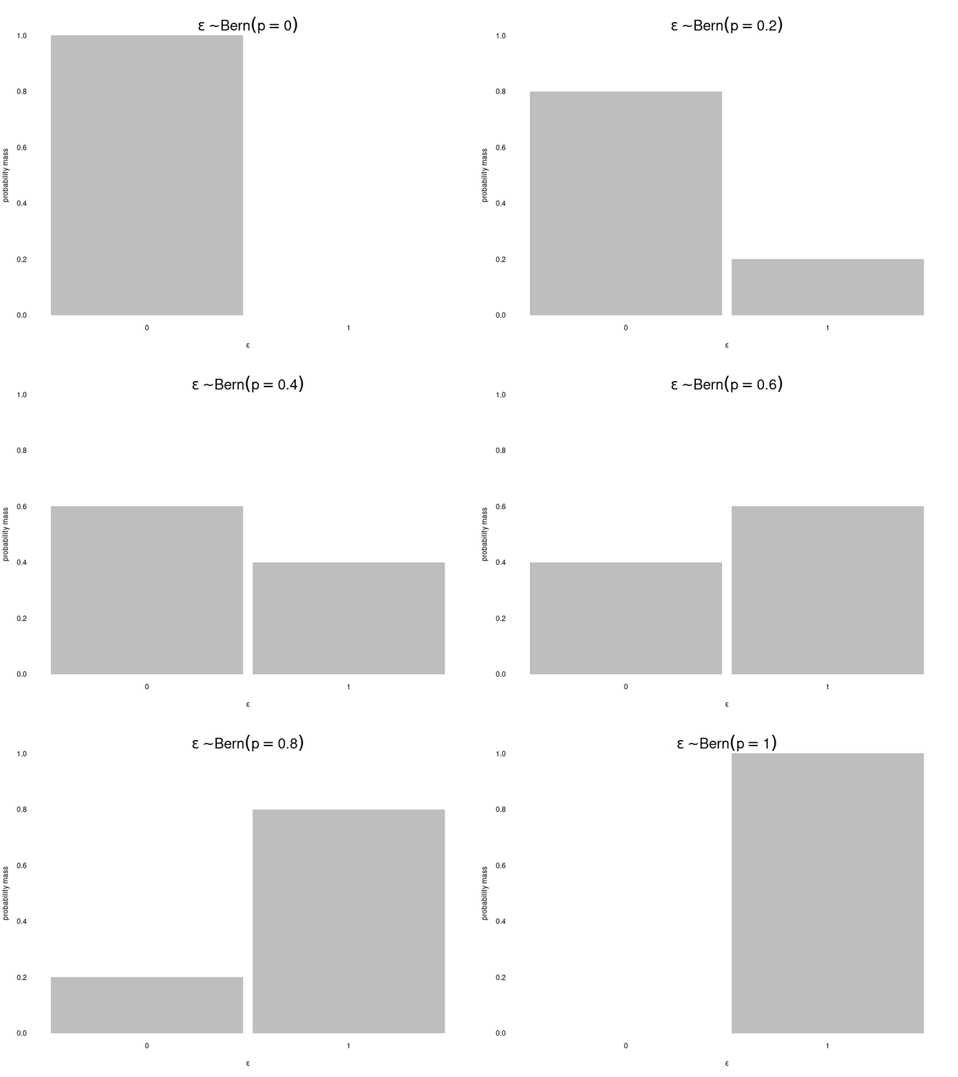
Probability distributions are denoted using the symbol \(\sim\). If we want to model an error variable as a Bernoulli distribution, we’d write \(\epsilon \sim \mathcal{Bern}(p)\). This reads as “epsilon is distributed as a Bernoulli variable, with parameter \(p\).”
The Bernoulli distribution is important, but is rarely directly useful because it only models a single observation. What if we expand our coin flipping procedure? We could flip a coin \(n\) times and count how many heads are observed. This sort of procedure is commonly modeled using the binomial distribution (another family). To notate that a variable follows a binomial distribution, we’d write \(\epsilon \sim \mathcal{Binom}(n, p)\), where:
\[ \begin{aligned} p &\in [0, 1]\\ n &\in \mathbb{N}\\ \epsilon &\in \{0, \ldots, n\}\\ P(\epsilon = k) = {n \choose k}p^k(1 - p)^{n - k} \end{aligned} \]
Notice that the binomial distribution family has two parameters: \(p\) and \(n\). \(p\) is the same probability as in the Bernoulli distribution; \(n\) is the total number of measured events (e.g., coin flips).
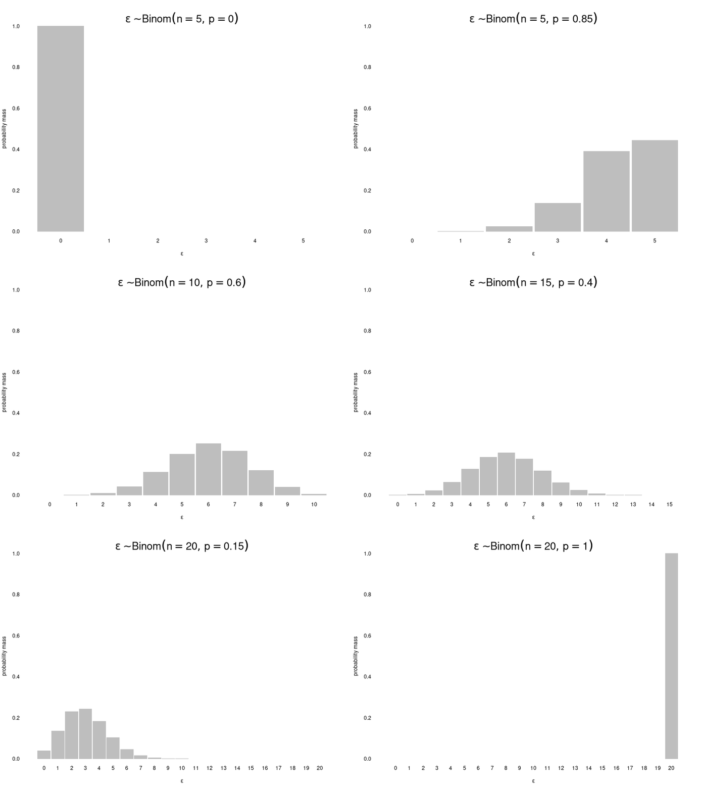
As before the binary variable we’re modeling could be any pair of observations; we could be counting heads, or musicians, etc. In this case, \(\epsilon\) isn’t representing the original variable (e.g., heads vs tails) but our counts of that variable.
What if we want to have more than two categories? For multinomial variables (more than two levels), the equivalent of the Bernoulli and binomial distributions are the categorical and multinomial distributions. These distributions require additional \(p\) parameters (\(p_1\), \(p_2\), etc.)—one for each level (minus one).
Normal Distribution
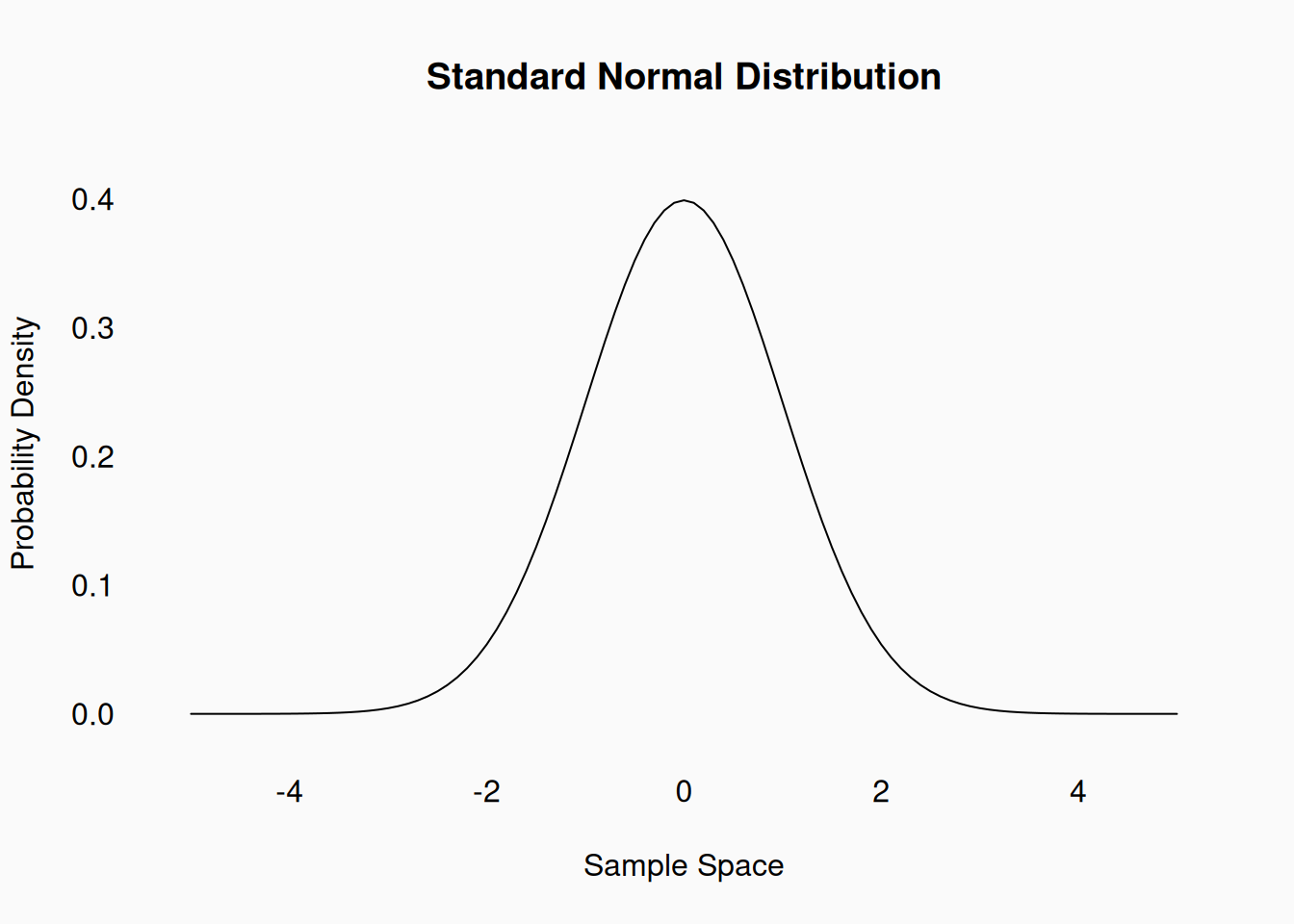
When dealing with numeric variables, the most commonly used probability model is the family of Gaussian distributions—also known as normal distributions. The normal distribution is defined over \(\mathbb{R}\)—a continuous and unbounded sample space. The standard normal distribution is a specific distribution, defined by this equation:
\[ \begin{aligned} x &\in \mathbb{R}\\ P(x) &= \frac{e^{\frac{-x^2}{2}}}{\sqrt{2\pi}} \end{aligned} \]
However, we can parameterize the full (infinite) family of normal distributions using two parameters: the mean (\(\mu\)) and standard deviation (\(\sigma\)).
\[ \begin{aligned} x,\mu &\in \mathbb{R}\\ \sigma &\in (0, \infty]\\ P(x) &= \frac{e^{-\frac{x - \mu}{2\sigma}^2}}{\sigma \sqrt{2\pi}} \end{aligned} \]
The key thing to note in this second equation is that, instead of \(x\) we have \(\frac{x - \mu}{\sigma}\). This means that the probability space is centered around \(\mu\) and scaled by \(\sigma\). Thus, the center of the distribution is \(\mu\) and the “width” of the distribution is controlled by \(\sigma\). If you measure the standard deviation of enough draws from a normal distribution, it will indeed match \(\sigma\).
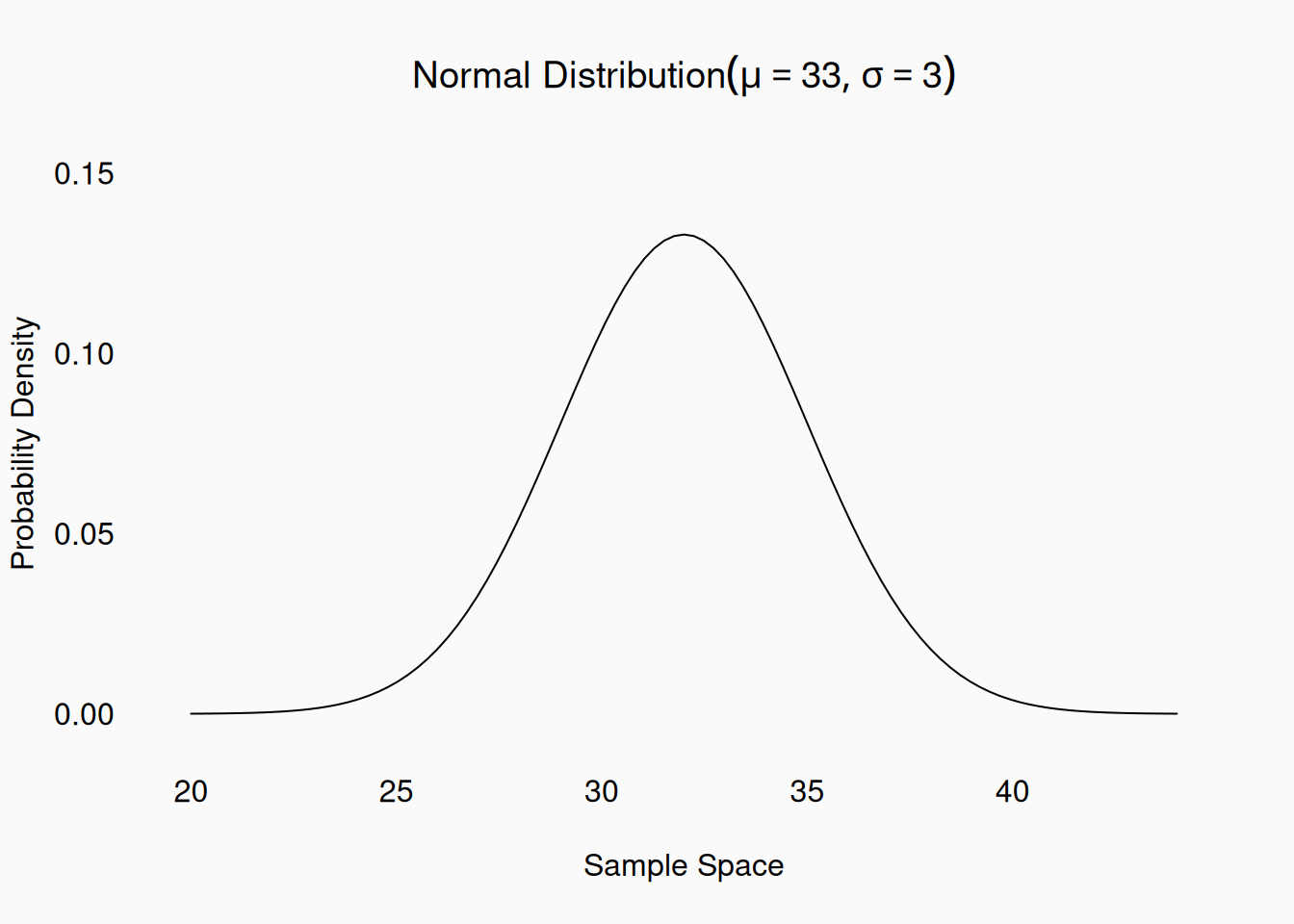
The notation for the normal distribution is:
\[ \begin{aligned} \epsilon &\sim \mathcal{N}(\mu, \sigma)\\ \epsilon,\mu &\in \mathbb{R}\\ \sigma &\in (0, \infty]\\ \end{aligned} \]
Other important distributions
The binomial, multinomial, and normal distributions are the most commonly used probability distributions in data analysis. However, there are many other useful distributions to be aware of, as they can be better models of certain types of variables or processes, or have other useful mathematical properties. All of these distributions have extensive, detailed pages on Wikipedia, which is an excellent reference for this sort of thing.
Count Data
The Poisson distribution generalizes the binomial distribution to \(n = \infty\). The Poisson distribution, for higher values of \(\lambda\), looks a lot like a normal distribution, but over discrete numbers.
\(\epsilon \sim \mathcal{Pois}(\lambda)\)
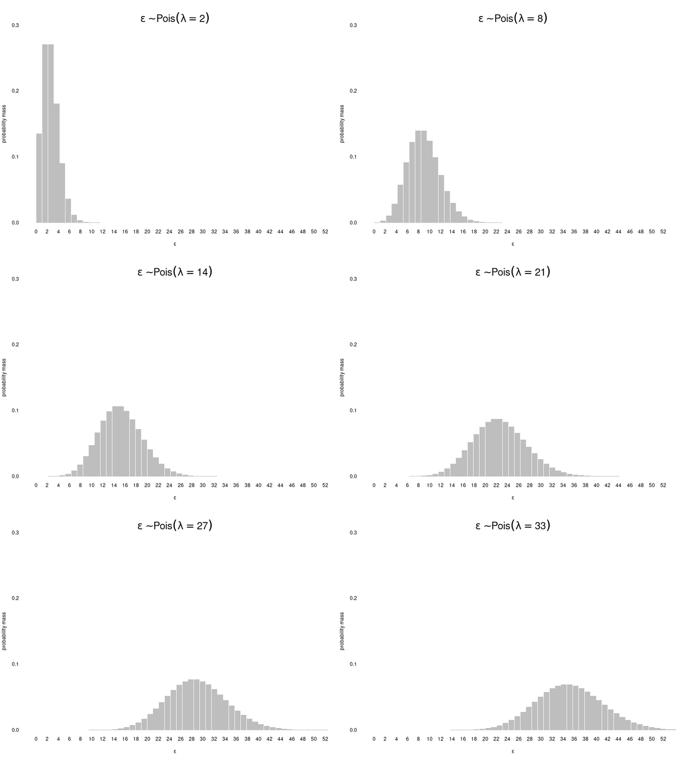
The Poisson distribution can be a good model of count data over time periods. For example, if you measured the number of people who log onto a music streaming site every minute, this would likely look like a Poisson distribution.
\(\lambda = E(\epsilon) = Var(\epsilon)\)
The \(\lambda\) (lambda) variable is both mean and variance of the Poisson distribution, corresponding to the average number of counts per time window. For example, if on average, 12 people sign onto our streaming site every minute, we might expect the distribution of counts by minute to look like \(\sim \mathcal{Pois}(\lambda = 12)\).
The negative binomial distribution is an alternative model of count data, which has the advantage of having two parameters, which allows it to have separate values for its mean and variance. It is also a generalization/extension of the binomial distribution. The negative binomial distribution is a good model of “the number of failures before a success.” For example, if you wanted to model how many attempts it takes a student to take on an ear-training quiz before they succeed and pass the quiz, the negative binomial could be appropriate.
\(\epsilon \sim \mathcal{NB}(r, p)\)
Bell shapes
The Gaussian (normal) distribution is the most common “bell shaped” distribution over the real numbers. However, there are a few other similarly shaped distributions which we use because they have other useful mathematical properties. Two important ones are Student’s t distribution and the logistic distribution, both of which we’ll learn a lot more about later in the book.
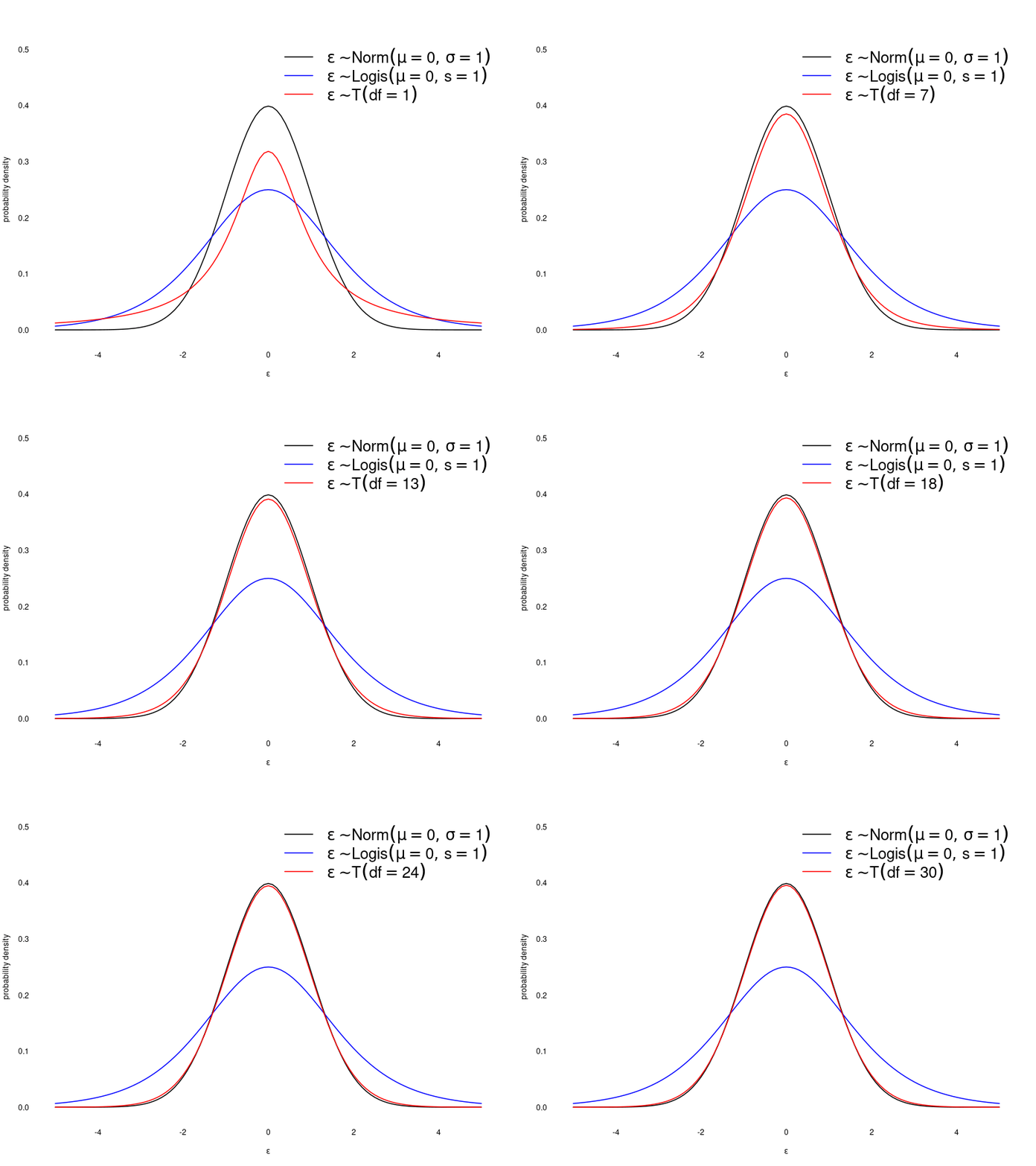
\(\epsilon \sim \mathcal{T}(df)\)
\(\epsilon \sim \mathcal{Logis}(\mu, s)\)
Proportions
The beta distribution is a useful distribution over the real numbers, bounded in the inclusive range \([0, 1]\). This makes it useful to represent things like proportions, success rates, and probabilities. In fact, it is often used to model the distribution of the \(p\) parameter in a binomial distribution—Yep, a distribution of distribution parameters!
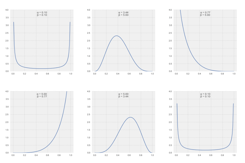
\(\epsilon \sim \mathcal{Beta}(\alpha, \beta)\)
The beta distribution is the conjugate distribution of the binomial distribution. “Conjugate distributions” are a statistical concept that we won’t really get into in this class, unless there is a lot of interest in Bayesian statistics. I’ll note that one of the many magical properties of the normal distribution is that it is the conjugate of itself.
The Dirichlet distribution extends the beta distribution to more dimensions, just as the multinomial distribution extends the binomial distribution.
Characterizing Random Variables
Every probability distribution is different. However, we can characterize any probability distribution in several, standard ways.
One way to characterize a probability distribution (or random variable) is its central tendency (a.k.a., “location”): values which get drawn a lot, or which draws tend to be “close to” or “centered” around. We can also characterize the dispersion (a.k.a., variability or “spread”) of a distribution, both regarding the magnitude and “shape” of the variability. Which central tendency and dispersion characterizations make sense depends on the type of variable.
Mode
The first measure of central tendency to consider is the mode—i.e., the most frequently observed outcome. The mode is the only meaningful “central tendency” for a categorical variable. However, if the number of levels is large, the mode is often not very useful. For example, you might observe a multinomial distribution with the following parameters:
| Rock | Reggae | Blues | Pop | Country | Jazz | Film | Classical | Metal | Punk | Funk | R&B | Folk |
|---|---|---|---|---|---|---|---|---|---|---|---|---|
| .14 | .04 | .09 | .15 | .13 | .08 | .03 | .03 | .04 | .07 | .05 | .08 | .06 |
The mode of this distribution is Pop, but Pop only occurs 14% of the time, so it is a pretty weak central tendency. The variation ratio is one way of quantifying this weakness, and thus the “spread” in a categorical distribution. The variation ratio is simply \(1 - P(mode)\); in the table above, it would be \(1 - .14 = .86\). In contrast, here is a different probability distribution over the same sample space, with the same mode:
| Rock | Reggae | Blues | Pop | Country | Jazz | Film | Classical | Metal | Punk | Funk | R&B | Folk |
|---|---|---|---|---|---|---|---|---|---|---|---|---|
| .12 | .02 | .02 | .67 | .06 | .01 | .01 | .01 | .01 | .01 | .01 | .01 | .02 |
The distribution is much more concentrated on the mode, so the variation ratio is much lower, at \(.33\).
For any continuous variable the mode is meaningless, as no precise value will ever occur more than once. However, we can identify the highest point where the derivative of a probability density function is 0.
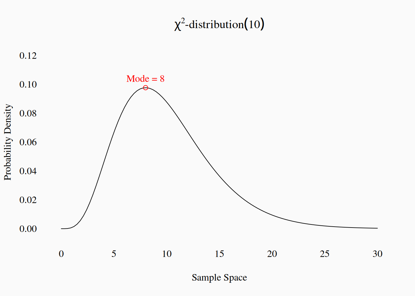
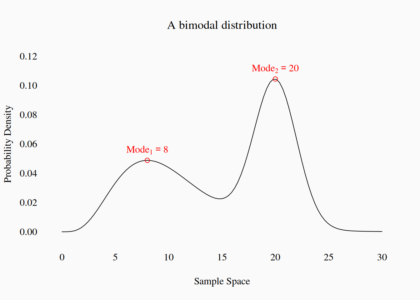
If a distribution has more than one peak, like this, we might describe it as bimodal, or multimodal.
Quantiles
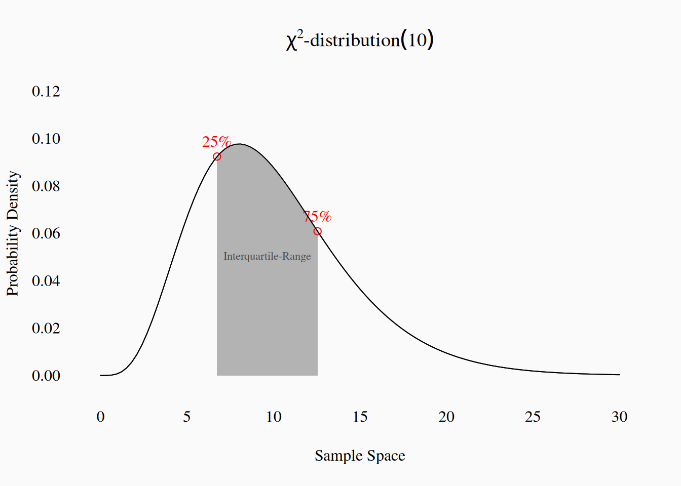
If our sample space is ordered, we can calculate quantiles. Quantiles are points in a distribution which divide the distribution’s probability mass into specific proportions. The most common quantile is the 50% quantile, more commonly known as the median, which divides the probability mass in half: half of observed draws are above the median, half are below. The median is thus a useful measure of central tendency, which only assumes ordinal structure. The next two most common quantiles are the quartiles (i.e., the 25% and 75% quantiles), which further divide the distribution into four equal masses. The interquartile-range is a very useful measure of dispersion, as it captures the “middle half” of the distribution.
Other common interquantiles are the 90% and 95% interquantile ranges:
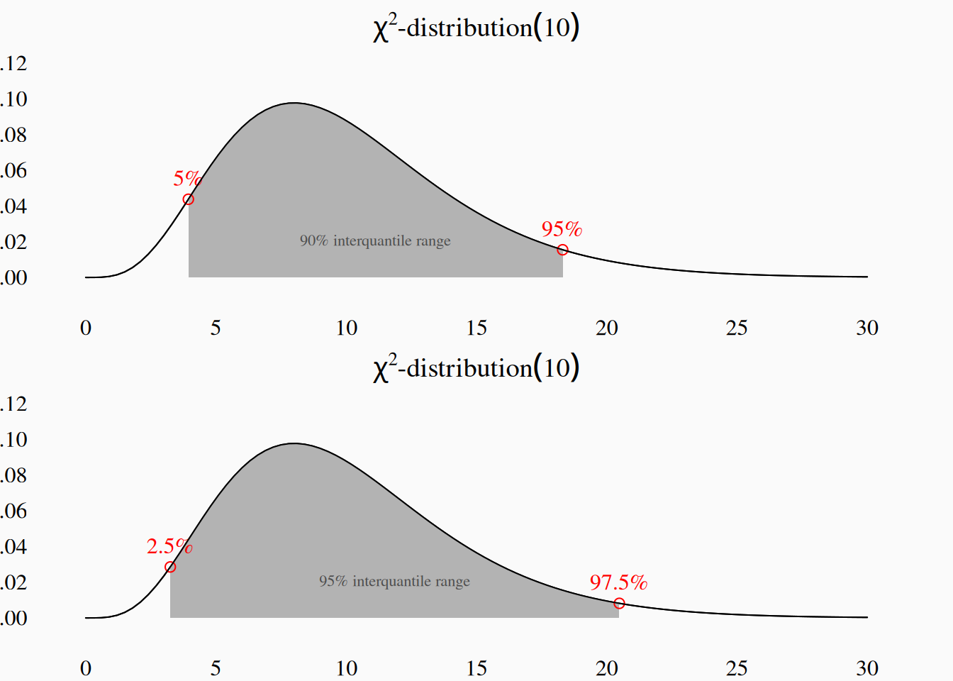
A final metric of spread to consider is the full range of values, from the 0% to 100% quantile. For the \(\chi^2\)-distribution we’ve been plotting, the full range is \((0, \infty)\); we say that this distribution has a lower bound at zero, but no upper bound.
Quantiles can also be calculated for discrete ordinal variables, but not always as precisely. For example, consider the following probability distribution over an ordinal scale:
| strongly dislike | dislike | somewhat dislike | neutral | somewhat like | like | strongly like |
|---|---|---|---|---|---|---|
| .01 | .02 | .09 | .2 | .37 | .26 | .05 |
There is no way of breaking this into two halves with 50% of the probability mass each. However, we could say that “somewhat like” is the median because it, and all lower values, account for 69% of the probability mass.
Mean
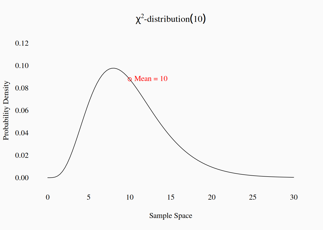
If our sample space is numbers on interval or ratio scales, we can use the arithmetic mean (\(\mu\)) as a measure of central tendency. The mean is the most important measure of central tendency in statistics. It is also called the expected value of a (numeric) variable: \(E(X)\). The mean is the sum (or integral) of all the values in the sample space, weighted by their probability.
The most common dispersion parameter for interval/ratio numeric variables is the variance, notated \(\sigma^2\) or \(Var(X)\). Like any good measure of dispersion, the variance captures how “wide” the error is around the mean. The variance of a distribution is the expected value (mean) of the squared deviations from the mean.
\[ \sigma^2 = E((X - E(X))^2) = Var(X) \]
Because the variance is built from squared deviations, the magnitude of the variance is not related in an intuitive way to the actual data scale. This means that, you can’t really visualize the variance of data very well. However, we can return to the scale of the original data by “unsquaring” the variance (i.e., taking the square root). The result is called the standard deviation (\(\sigma\)), which can be visualized on the scale of the original data:
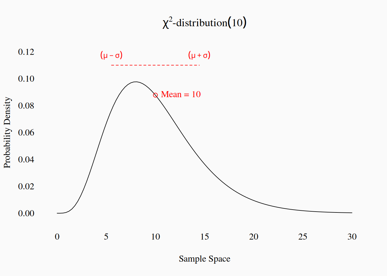
It is very common to normalize distributions by subtracting the mean and dividing their values by their standard deviation, forcing the data/distribution to have a mean of zero and a standard deviation of one. However, this only makes sense for values on a ratio scale. It wouldn’t make sense to normalize degrees Farenheit (\(^{\circ} F\)) but degrees Kelvin could be normalized. A common normalized dispersion metric, for ratio-scale numbers, is the coefficient of variation \(\frac{\sigma}{\mu}\). Similarly, other forms of “mean,” like the geometric and harmonic means, are only meaningful on a ratio scale.
Symmetry
Some probability distributions are symmetrical around their mean. For example, the normal distribution is symmetric. However, other distributions can be asymmetrical, and there are a few common approaches to quantifying this asymmetry.
The variance (\(E((x - E(x))^2)\)) is based on the squared deviations from the mean. If we instead calculate the expected value of the cubed deviations from the mean—\(E((x - E(x))^3)\)—, we get a metric called skew. Symmetrical distributions have \(skew = 0\). The standard skewness metric, Fisher’s moment coefficient of skew, normalizes the skew to an abstract (unit-free) scale by dividing the deviations by the standard deviation before cubing: \(E((\frac{x - E(x)}{\sigma})^3\).
The most intuitive way of thinking about skew, is that in a skewed (asymmetrical) distribution, the median and mean are different. This suggests a simpler, non-parametric metric of skew: \(\frac{mean - median}{standard\ deviation}\). This “median skewness” can range from -1 to 1.
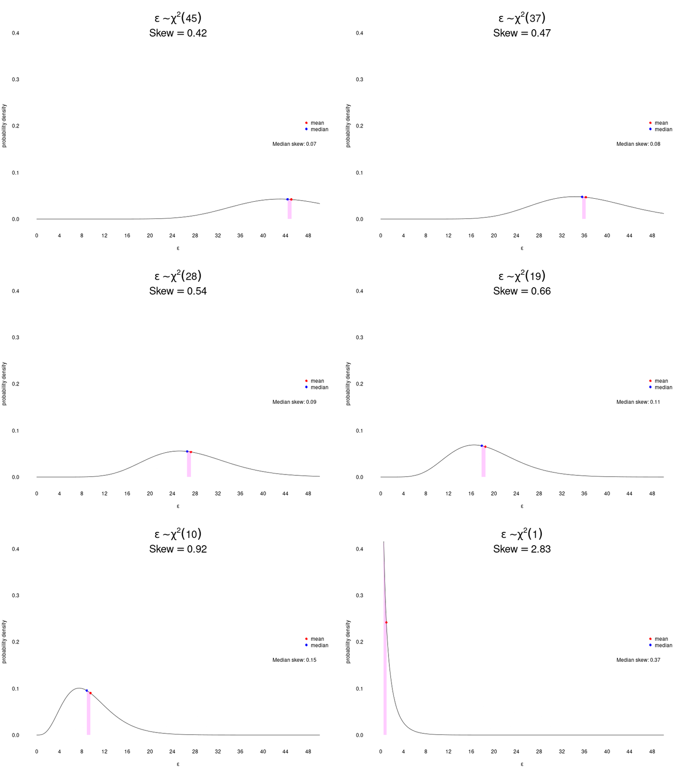
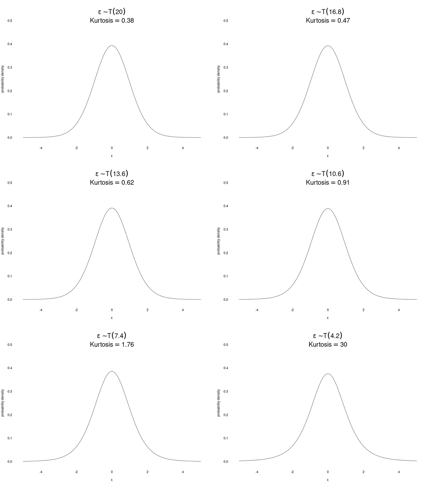
If we go one step farther and calculate the average (normalized) hyper-cubed deviations—\(E((\frac{x - E(x)}{\sigma})^4)\)—, we get the kurtosis. Kurtosis reflects how much of a probability distribution’s mass is spread in its tails: the extremes at either end of the distribution—i.e., rare events. The normal distribution has \(kurtosis = 3\), so any distributions with more frequent extreme values than the normal distribution will have “excess” kurtosis higher than that.
Multi-modal problems
Notice that central tendencies, and all the measures “around them” (variance, skew, kurtosis), assume a unimodal (one mode) shape. If we have something like this
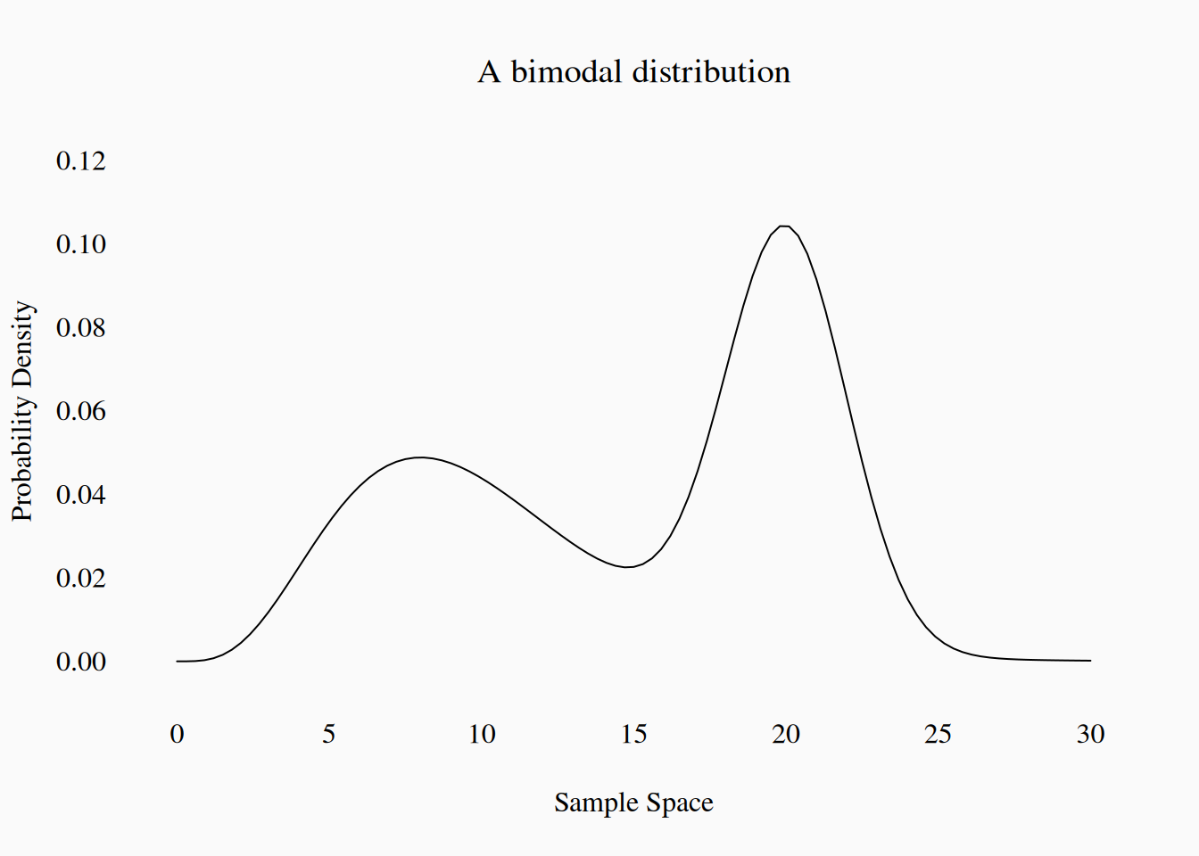
we can still calculate the mean, variance, skew, etc., but we should regard them with a grain of salt right?
Entropy
A final useful measure of probability dispersion is Shannon entropy—also known as information entropy or just entropy. Entropy is useful because it isn’t “centered” around anything, and thus can be applied to any distribution, either categorical or numeric. Entropy is basically the average (log) probability of draws from the distribution: we can think of this as how “surprising” observations are, on average. Claude Shannon’s original paper (1948) on entropy is one of the most cited scientific papers ever published, and founded the field of information theory. Shannon described entropy as the average amount of information conveyed by the random variable.
The entropy of a variable is usually denoted \(H(X)\), where \(X\) is the random variable.
\[ H(X) = E(-{\log P(X)}) \]
For a non-random variable, where each observation is always the same (\(p = 1\)), entropy is 0. As a variable gets more and more dispersed, and observations are more uncertain, the entropy increases.
Entropy is a nice measure of how “flat” a distribution is. Consider again our two different multinomial distributions from above:
| Rock | Reggae | Blues | Pop | Country | Jazz | Film | Classical | Metal | Punk | Funk | R&B | Folk |
|---|---|---|---|---|---|---|---|---|---|---|---|---|
| .14 | .04 | .09 | .15 | .13 | .08 | .03 | .03 | .04 | .07 | .05 | .08 | .06 |
| .12 | .02 | .02 | .67 | .06 | .01 | .01 | .01 | .01 | .01 | .01 | .01 | .02 |
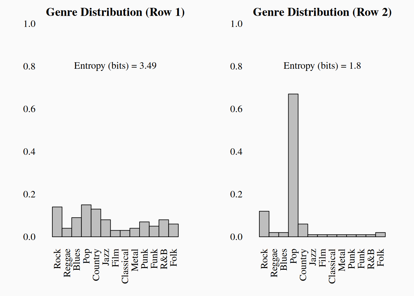
The right (Row 2) distribution has a lower entropy, because it is much more concentrated on a few values (especially Pop). When we draw from this distribution, more than half the time we observe Pop, so we aren’t surprised much. We do occasionally get surprised by a rare draw of Folk or Blues, but only very rarely—most of the time, we see the commonplace Pop. In contrast, when we draw from the left (Row 1) distribution, every observation is a bit of a surprise, so the entropy is higher.
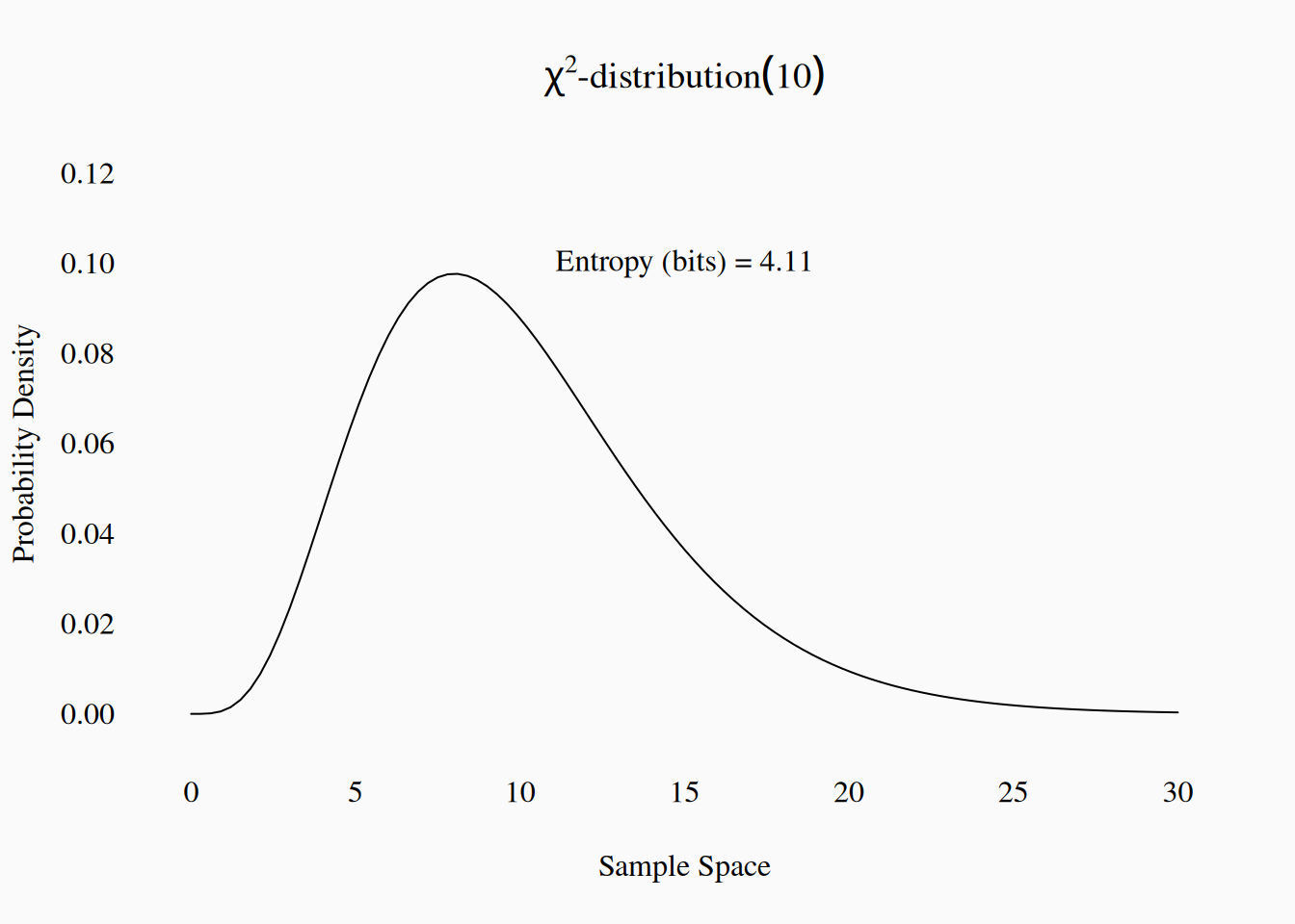
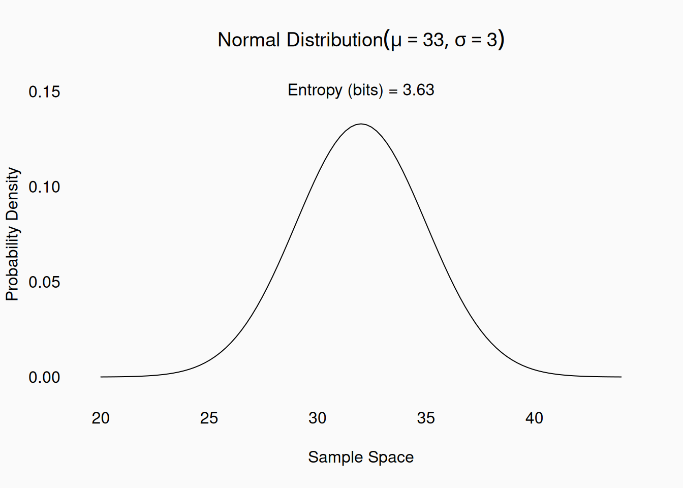
Entropy can also be calculated for continuous variables. Here are a few examples:
Entropy units
Entropy can be calculated with different bases for the logarithm. The most common approach is to use base-2 logarithms; When using base-2 entropy, the units of entropy are called bits.
Consider again our (fair) coin flip probability distribution from above. The base-2 entropy will be:
\[ H(\texttt{Coin Flip}) = -\frac{\log_2(.5) + \log_2(.5)}{2} = -\frac{(-1) + (-1)}{2} = 1 \]
Thus, a fair coin flip has one bit of entropy. A nice feature of entropy is that it sums (if the variables are independent); this means that the entropy of the distribution of two independent coin flips is two bits; For three independent coin flips, it’s three bits; and so on. Every additional (independent) coin flip adds one bit of entropy. This means that you can always interpret \(N\) bits of entropy as being equivalent to flipping \(N\) coins.
Other entropy units include “nats” (using natural log, with base \(e\)), and dits (base-10 log). One dit is equivalent to a 1-in-10 chance average; two dits is equivalent to a 1-in-100 chance average; etc.
Operational Assumptions
When we use a probability distribution to model error in our measurements, we are essentially incorporating this into our operational definitions. We often assume simple probability models because they are convenient, easy, standards. For example, the vast majority of statistical tests assume that error is normally distributed. As conscientious researchers, we should always consider the content validity of our error models, and the numbers we use to characterize them.
Once common (potential) problem is using normal distributions to model variables that are bounded. A normal distribution’s sample space is all of \(\mathbb{R}\), so it can always range from \(-\infty\) to \(\infty\). It is very common to work with operationalized variables that are bounded: for instance, a user-rating using a slider between 0 and 100, or proportions like “the proportion of listeners who like to listen to sad music.” A normal distribution, is in principle, not a good model for this sort of data. Still in practice, it may or may not be a problem to assume a normal distribution here. For example, consider this sample of data, and a normal distribution model which I am superimposing on it:
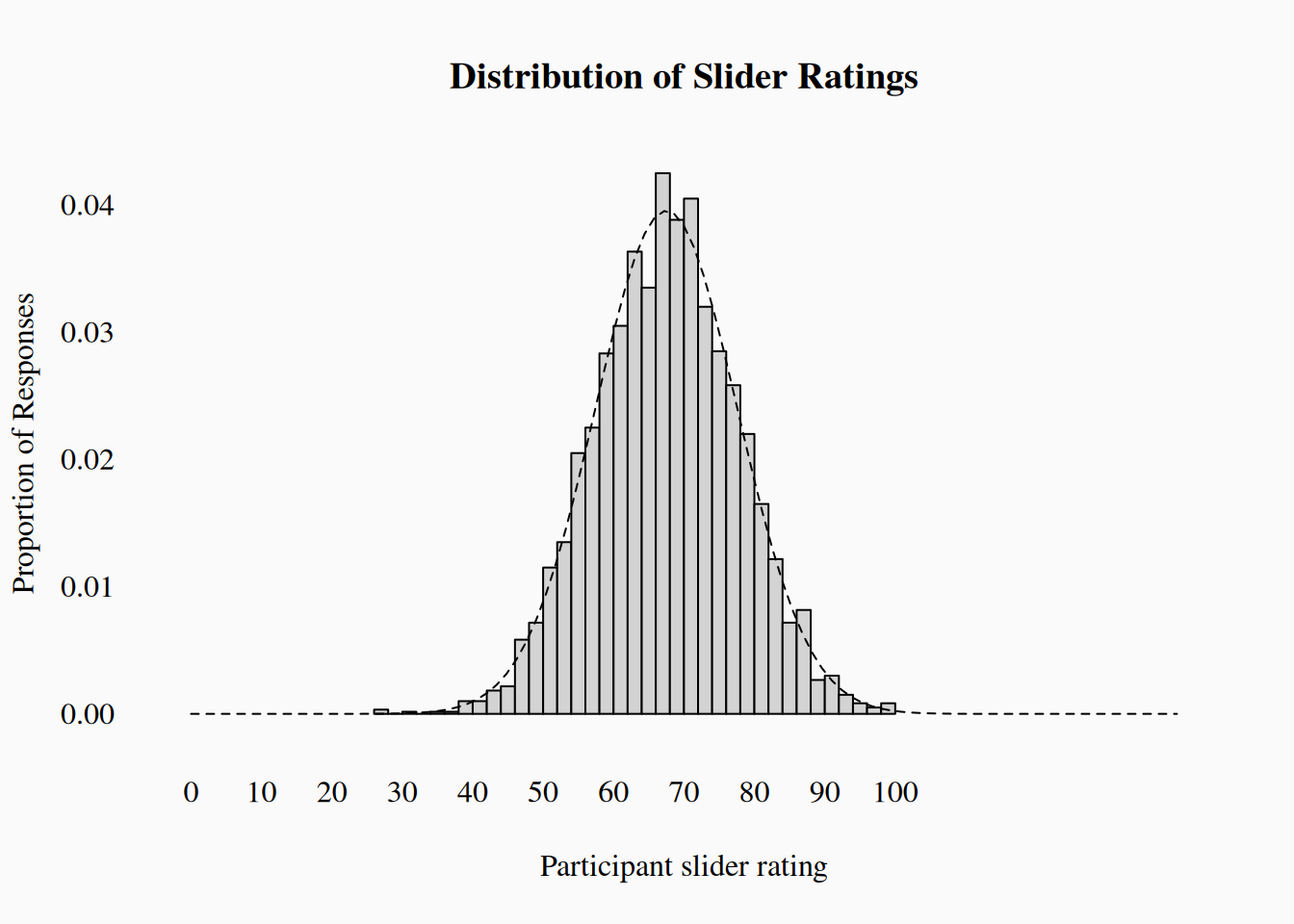
That’s not so bad. The right tail is sort of cut off, but it’s probably not a problem. But what about this data?:
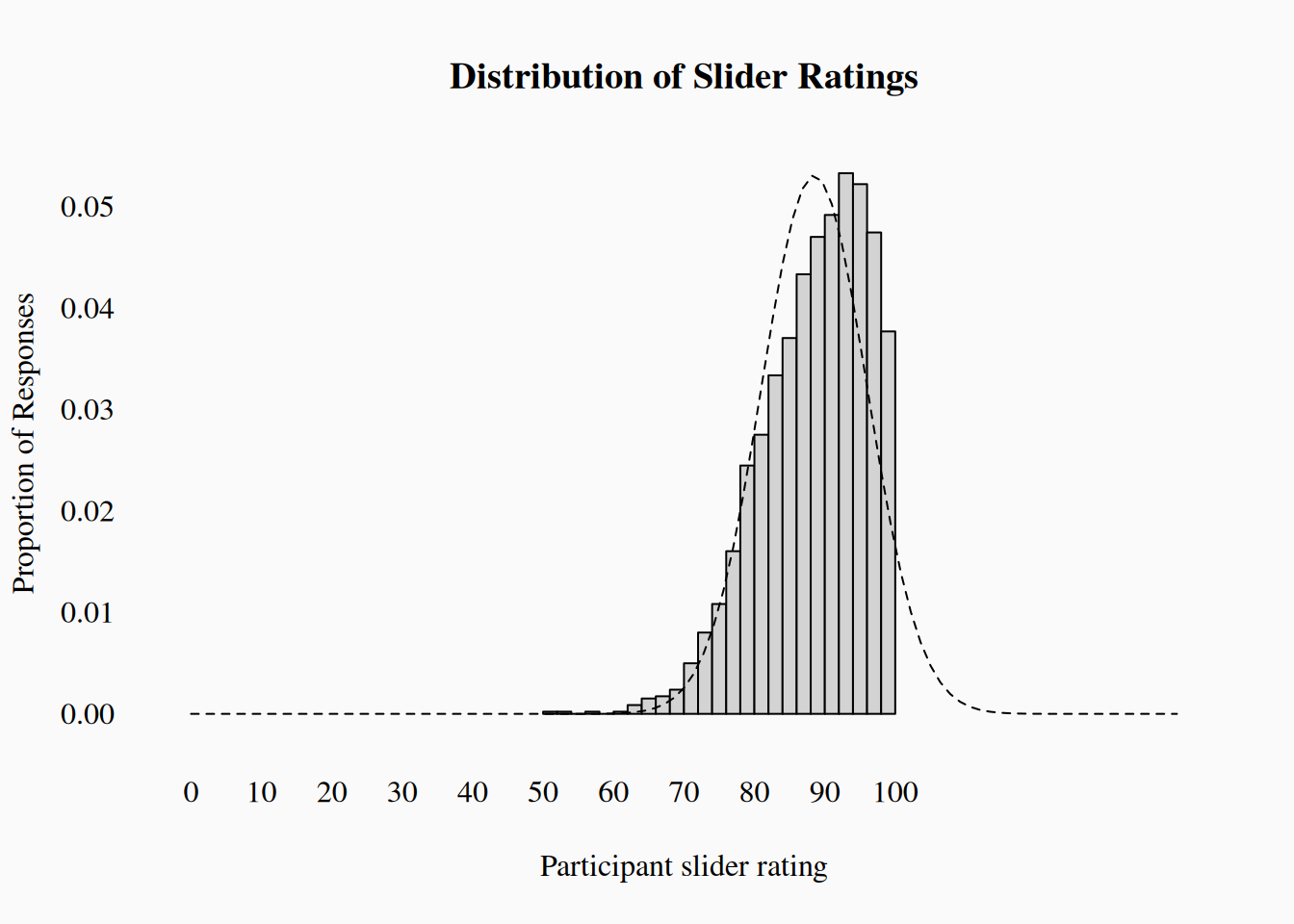
That normal distribution seems much less plausible now! We might want to consider an alternative probability model.
We might also consider when it makes sense to consider an operational measure to be “really” continuous. For example, does the slider we are using record fractional positions, like \(79.2\), or just whole numbers? If there are a hundred positions, its probably safe to “pretend” the data is continuous. If not, maybe a discrete distribution like the Poisson or negative-binomial would be more appropriate.
As always, it will take some judgement to decide when a probability model is a valid model of your variables. There is no easy answer.