
44 Data Analysis
(Modified on 2026-08-12)
857 words
45 Data Analysis
Science is the synthesis of rationalism and empiricism—theory and data: formally recorded measurements (observations) of the world.
What is the role of data in science? Data can inspire new ideas, new theories, new questions, new hypotheses. More importantly, data can be used to test theories. Data, if gathered and analyzed validly, allows us to evaluate and (potentially) falsify our claims.
Speak for Yourself
Inducing knowledge from data is the basis of empiricism. It is tempting—and all too common—to think that this process is “objective.” That we can simply sit back and “let the data speak for itself.” But this is not the case. Data doesn’t speak for itself.
Data is “objective” only in the sense that we cannot control what it will be before we gather/measure it. The exact result of each measurement must be outside of our control—This is what makes newly-collected data a useful tool to test hypotheses. However, as we know, we decide how data is sampled, defined, and recorded:
- If you are researching the relationship between gender and music…
- How many categories (and what) gender categories appear on your questionnaire?
- How do you define each gender category?
- How do you measure gender?
- If you are doing a study of musical intervals…
- Do you ignore register?
- What tuning system do you assume?
- How are vibrato and glissandi accounted for, if at all?
- If you are testing a new machine-learning system:
- Which system do you compare it to?
- Which evaluation metrics do you use?
- Which hyper-parameters do you test?
Data and data analysis are always shaped by these sorts of subjective decisions. What’s more, the process of inducing knowledge from observations is not “objective” either; There is no method which simply extracts “objective truth” from data. Data never “speaks” at all—we interpret data.
Data Analysis Goals
When it comes time to analyze your data, your goal should not be to extract information from your data. Or even to discover unknown patterns that are “in” the data. Your goal should be to question patterns that appear to be in your data. Criticise the data; Be a skeptic. This is how you create compelling scientific rhetoric about your data.
All data includes random and systematic error. Unfortunately, humans are very good at seeing patterns in randomness—a pattern might be apparent to us, even if there is not “true” underlying cause for it. In particular, when we want to find patterns, or anticipate seeing specific patterns, it is easy for us to “find” them (confirmation bias). My mind is prone to positives
This is why the default skeptical perspective with which we regard any and all data is: “it could just be noise.” This is the starting point of any data analysis. When it comes time to write the results or evaluation part of a research paper, your job is to try to show that your data is just noise.
- Your machine learning model performs 2% better than the previous state-of-the-art model?
- It was probably just lucky chance. Or maybe you have done something to bias the performance in your model’s favor. That’s what you aim to prove.
- Your musician participants averaged higher “openness to experience” scores than your non-musician participants?
- It was probably coincidence that you recruited some open-minded musicians. Or maybe your operational measure of openness correlates with some aspect of musical training. That’s what you aim to prove.
If you can’t demonstrate that noise or bias is the explanation, then claiming that the model really does perform better will seem plausible to readers.
This does not mean that “it could be noise” is the only skeptical claim we can make about data. Just an obvious one.
There are many standardized approaches to analyzing data. All approaches are based on skepticism towards the analysis and conclusion. All approaches make it harder for us to make positive claims about our data: That is the point.
Modeling data
All data analysis relies on theoretical models:
- Models of the constructs our variables represent:
- Number of levels; Dimensionality; Mathematical properties (ordinal, interval); etc.
- Models of the measured variables and how they relate to underlying construct:
- How true levels map to measured levels; How is error distributed; etc.
- Models of relationships between variables:
- Linear; quadratic; interactive; meditative, etc.
Models are formal representations of theoretical knowledge. The best way to specify formal models in a precise, potentially falsifiable way, is with math! In particular, representing models as variables in linear equations, with relationships between variables expressed using addition or multiplication by various parameters. Statistical models are mathematical models which include stochastic elements—i.e., random variables—, allowing us to think formally about randomness and error. However, not all formal models are mathematical (or linear): other modeling approaches can be more structural or descriptive. For example, flow diagrams, hierarchical groupings, etc.
The models that we assume always shape our analyses, to some extent. However, in different forms of inquiry, the relationship between theoretical knowledge (deduction) and empirical data (induction) can differ.
In theory-driven analyses, we use a priori theoretical models to make sense of data. By superimposing a priori knowledge on our data, we can better understand what we are observing.
For example: If we go to analyze F0 pitch-contour data for vocal music, we can use our theoretical knowledge to recognize errors (negative frequencies or F0 above \(1_{kHz}\)), octave equivalent passages, or the difference between vibrato and actual melody. Conversely, we can use data to test—and potentially falsify—our a priori theories.
In totally theory-driven analyses, we need to precisely specify our models in advance, so we can apply them to our data and recognize when data conflicts with them.
In exploratory analyses, we use data to fill in the gaps in our current theories, or help us develop entirely new a posteriori theories/models of the data. By making fewer assumptions about data, we can avoid biasing our results to match our expectations.
In totally exploratory analyses, we can (and should) explore many possible models of the data:
- Could the relationship between
XandYbe linear, quadratic, or cubic?- I don’t know, try them all.
- Could there by an interaction between any of the variables
X,Y, andZ?- Let’s see!
The greatest challenge is that there are always a lot of potential relationships and models to explore—too many to try them all—and many of them will fit the data equally well. This is what makes it hard to make strong claims based on exploratory analyses.
- Could the relationship between
Whatever analytical approach we take, it is always important to be honest with our readers, and ourselves, about which theoretical ideas and models are a priori and which are a posteriori (or post hoc).
Descriptive Analysis
Often the first step when analyzing data is to describe our data. Descriptive analysis tends to be less theory-driven, making only basic assumptions about our variables. However, descriptive analysis is also an opportunity to use our theoretical knowledge to identify problems with the data (measurement errors, missing data, etc.).
Imagine this research scenario: I hypothesize that older people prefer listening to music at quieter volumes and I gather appropriate data (age and preferred listening \(dB_{SPL}\)) to test this hypothesis. What would be my analysis approach? As a default, I would probably plan (a priori) to model the relationship between age and listening level as a linear function, with normally-distributed error. Something like:
\[ \begin{aligned} ListeningPreference_{dB\ SPL} = X_0 + X_1 * Age_{years} + \epsilon\\ \epsilon \sim \mathcal{N}(0, \sigma)\\ \end{aligned} \]
However, during my descriptive analysis I plot the data and see this:
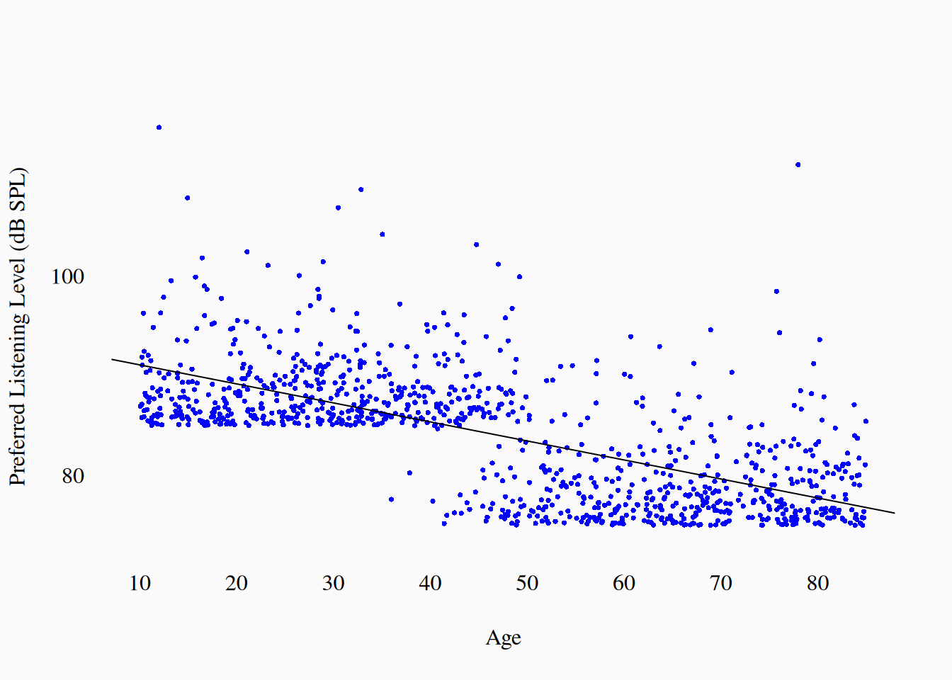
Clearly, a linear trend doesn’t seem to be a great description of this data; Rather there seems to be an abrupt drop in preferred level around age 50. After observing this, I think it would be better to model this data using a binary age variable (\(Age_{years} > 50\)). (The statical test would be a \(t\)-test instead of a linear regression.) I also note that the error seems to be skewed a lot towards higher values:
Warning in sqrt(resid): NaNs produced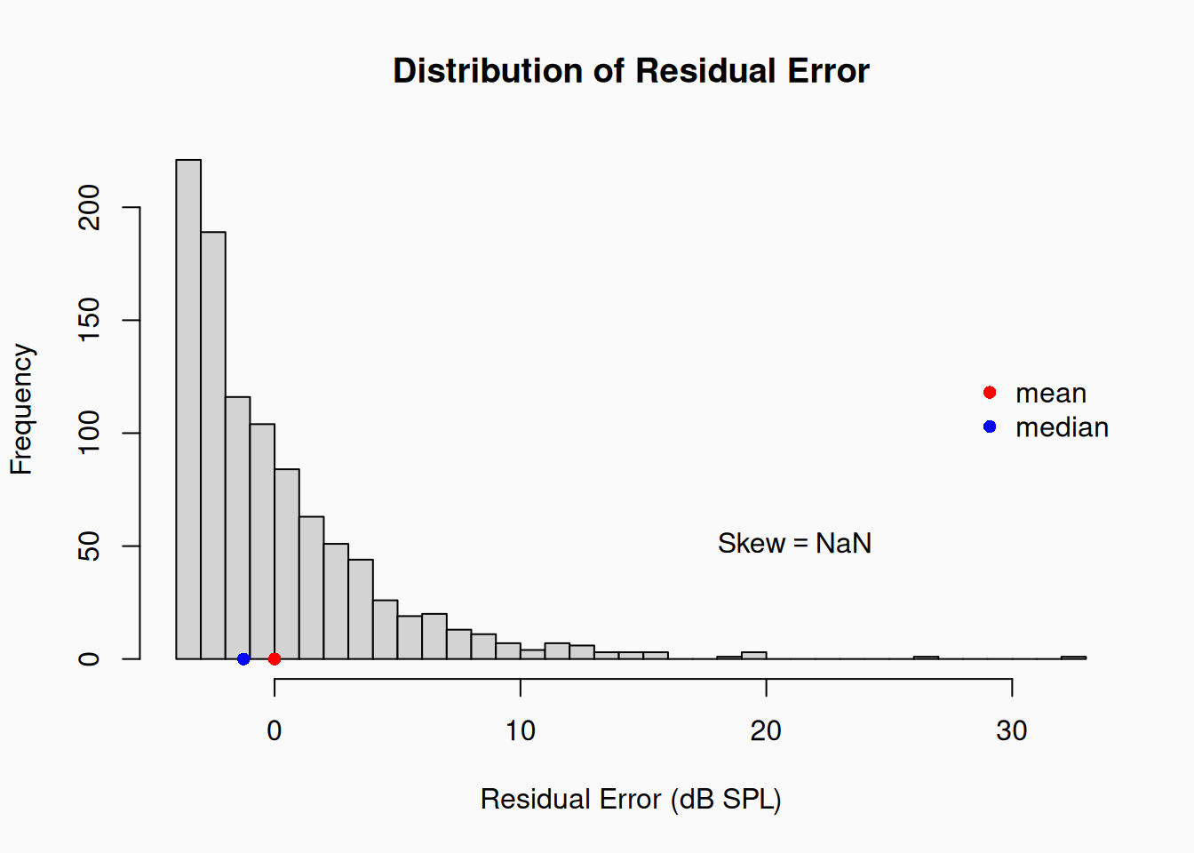
Thus, it might be appropriate to use a different error distribution than the (symmetrical) normal distribution. My descriptive analysis has helped me refine and improve my model of the data, which will hopefully lead to better (more valid) conclusions and claims.
Notice that, in the scenario above, I’m making changes to my research methodology post hoc. As we know, this might be a problem.
- If I specifically hypothesized that the relationship between listening preference and age would be linear, then I’d need to acknowledge that my hypothesis is inconsistent with this descriptive analysis, and perhaps falsified.
- For example, if my theory was that loud listening preferences are caused by testosterone, and since testosterone levels (in both men and women) gradually drop as we age, that preference for loudness should also drop gradually. In this case, my descriptive analysis seems to conflict with the theory and I can’t ignore that—I need an alternative theory that would explain a sudden change around age 50.
- Similarly, if I specifically hypothesized that listening preferences would be symmetrically distributed, then I’d need to acknowledge that my hypothesis is inconsistent with this descriptive analysis, and perhaps falsified.
It is fine to use post hoc reasoning to modify our analyses or claims, as long as we acknowledge this explicitly. We can say something like:
Our hypotheses and assumptions about how the data would be distributed were not consistent with the data. We thus pursued a different post hoc analysis strategy, using a binary-age variable (cut off at age 50) and asymmetrical error distribution.
Now, in many inquiries, our hypothesized models simply aren’t that specific. For example, we might hypothesize that older people like music quieter, but have no specific idea about whether there would be a linear change, a quadratic change, or some kind of discrete shifts. If this is (genuinely) the case, then it is fine to use our descriptive analysis to make decisions about analyses/claims. As long as we aren’t pretending something is a priori when it wasn’t, there is no problem.
Note: Reviewers will be suspicious about what research decisions/models are and aren’t a priori. The only way to decisively convince a reviewer is to be extremely honest and upfront about what decisions were post hoc. If you clearly say “X, Y, and Z were post hoc,” reviewers will be inclined to believe you when you say that “I, and J were a priori.”
If our inquiry is entirely exploratory, then obviously everything we do is a posteriori and there is no reason to sweat these details too much. Maybe I just gathered a bunch of data about listening preferences and spent some time combing through the data until I stumbled across the (apparent) change in loudness preference with age. An exploratory finding like that is harder to validate, and leads to a weaker claim (compared to a hypothesis-driven approach), but is still interesting. I could also use the exploratory observation (change in preferences at age 50) to motivate my next experimental research project—the explore then test paradigm.
Inferential Analysis
We generally don’t want to just describe our data. Our data is only a (small) sample of (imperfect) operational measurements of the universe. Rather, we want to use our data to make inferences about the universe—the “population” of constructs beyond our data. In inferential analysis, we propose that our data models are actually models of true causal relationships/processes in the real-world. The goal then, is not just to model the data at hand, but to claim that our theoretical model actually represents true knowledge about the universe.
Inferential analysis is the main goal of most scientific inquiries. Whereas descriptive analysis is a useful means to an end, inferential analysis is the actual end goal: generalizing our claims to the real world—the population beyond our sample. The key thing we have to argue in our inferential analysis is that our methods/models have external validity.
Case study
In our study of “tempo-stability” in music (Condit-Schultz and Clark 2024), we hypothesized that rock, blues, and country music would show a drop in tempo-stability at some point in the last quarter of the 20th century. We didn’t know how much it would drop, when it would drop, or what the temporal shape of the drop would be; However, we did weakly hypothesize the drop would happen around 1980. When we looked at our data, we saw this:
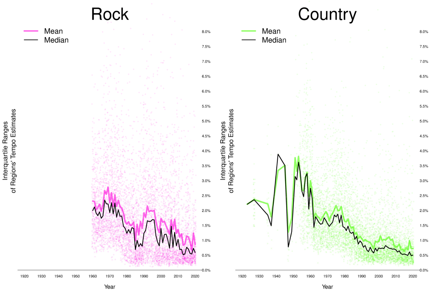
The year 1980 doesn’t seem nearly as important in these graphs as we guessed it would be. Still, the first thing we did was test whether tempos were slower, on average, after 1980 than before (and they were \(p < .05\)). Since the historical curves are so messy and complicated, and we had no a priori hypothesis about the contour of the historical change, we chose to do something really simple: a binary cut off comparison (\(t\)-test) between tempos before and after 1980. Thus, we didn’t downplay or abandon our a priori hypothesis, even when the descriptive analysis suggested otherwise—we owned the (obvious) discrepancy between what we expected and what we saw. However, after this first (dumb) test, we were then free to do a bunch more post hoc analyses.
Ultimately, we made the inferential claim that tempo-stability really has (in the real-world population of rock/country/music) gotten more stable over time, and that tempos were more stable after 1980. However, we avoided making any strong claims about the historical contour of tempo-stability changes, or about differences in when rock and country music changed their stability. We simply shared our descriptive analyses (including the graph) above, and allowed our readers to make their own conclusions. Hopefully, somebody else will eventually pick up the torch and run a theory-driven study to confirm or disconfirm that, for example, country music got tempo-stable later than rock music.
Applied Analysis
In applied research, successfully modelling “true” relationships in the universe isn’t always necessary. If an analytical model produces accurate predictions, it can be useful even if it is an “incorrect” model of the real world. For example, if older people really prefer quieter music, we might program our music-player apps to use a lower default volume level for older users, and we don’t need to know why they prefer music quieter (lack of testosterone?), just that they do.
Of course, just because age predicts loudness ratings in our sample doesn’t guarantee that it will work outside our sample. Thus, even in applied settings, we still care about external validity: we want to infer (generalize) from our sample to the population of (potential) future observations. The difference is that we don’t necessarily care about the internal validity—we don’t care about why the model works (internal causality), only that it will work for future cases.
Note: Though we often refer to machine-learning (ML) “models,” most such models are not really models of anything, per se. Most ML systems are black-boxes and don’t even pretend to make claims about how things “really work” outside the model. The internal workings of a ML “model” may or may not map to real-world relationships, and we don’t necessarily care if they do, so long as the input-output mapping is accurate.
The use of the term “model” was inherited from statistics, where models are taken to be real models of the world and where we do aim to justify the internal validity of models.
Standard Analysis Approaches
There are many “standard” approaches to analysis, which we will learn about in coming chapters. For example, standard visualizations, statistics, statistical models, and classification evaluation criteria. Using standard approaches—even though they are all imperfect—is a good approach, or at least a good starting point, because they are familiar to and well-understood by your reviewers. It also takes the burden of justifying all your analysis decisions off of your back. You can also copy (and cite) non-standard analysis approaches from specific papers, if they make sense for your project.
Here are some examples of extremely common modeling assumptions:
- That any numbers we have measured behave like real numbers (\(\mathbb{R}\)) on a linear, ratio scale.
- That error in our numeric variables is normally distributed, with equal variances.
- That false-positives and false-negatives are equally important.
- That Likert-type measurement items are an interval scale (not ordinal).
- That our data points are sampled independently.
It’s very likely you will make these assumptions in many of your own research analyses. However, it’s still important that you think about whether these assumptions are really valid for your research: is the data normally distributed? Is the measurement on a ratio scale? Etc. Generally, people can and do get away with making these assumptions without mentioning them; However, it always makes your rhetoric stronger if you explicitly acknowledge these assumptions. All you have to do is throw in a quick “…assuming the residuals are normally distributed” or “…if we treat the Likert-items as an interval scale” to make it clear you know what you are doing. Good researchers are always explicit about their assumptions.
Mantras
Data doesn’t speak for itself
Data is not objective; Analyses do not just “pop out” of the data. Data sampling, collection, parsing, munging, analysis…all are influenced by your subjective decisions. Data is interpreted by researchers.
Tortured data will confess to anything
It’s not true that “statistics can prove anything,” but it is possible to manipulate data in ways that deceive yourself and others. Create a data analysis plan. Do not exclude outliers, normalize data, set conditions for excluding participants, or introduce post hoc tests without some principled prior reasoning. Be honest in reporting the analyses you carry out. Don’t hide multiple tests.
Search for noise in the patterns
You might think data analysis is about uncovering patterns—but finding patterns you want to find is easy. The real problem is knowing whether a pattern is real. Since science means trying to prove ourselves wrong, the goal of analysis is to show the pattern isn’t there: make an honest, skeptical effort to explain away any correlation you observe before you believe it.