29 Data Independence
(Modified on 2026-08-11)
2,304 words
Suppose you were carrying out a telephone-based survey whose aim is to sample likely voting behavior for an up-coming election. Using an auto-dialing system, you are connected to successive random telephone numbers from certain area codes. Once you make contact, you ask the survey participants: (1) whether they are eligible and likely to vote in the election and (2) which candidate they are likely to vote for. You find that most telephone calls are unsuccessful: either no one answers, or the person is unwilling to participate. You are pleased whenever you encounter a cooperative respondent. As you complete your conversation with one person, you hear another voice in the background—it is the respondent’s husband. Eager to recruit another participant, you ask whether it would be possible to speak with the person’s spouse. They agree, and so you are able to collect data from two people rather than just one.
Savvy researchers discourage this sort of behavior. People who live together share many things in common—including attitudes. For married couples, both spouses are likely to share similar political views. Collecting data from two people who live together is much less useful than collecting data from two unrelated people. When collecting data this way, the results will appear more uniform than would occur in a proper representative sample. The data collected from 50 couples is less representative than the data collected from 100 independent people.
Often when we sample data, it is not feasible to sample every single data point separately: rather, data is found stuck together in natural “clusters.” This is called cluster sampling. Cluster sampling as a sampling procedure is sometimes the only feasible way to get sufficient amounts of data.
Sampling families (including married couples) is one example of cluster sampling, but there are many other examples:
- To sample pieces of classical music, we could sample datasets of scores by Mozart, Bach, Brahms, Beethoven, and Schubert.
- We might end up with a sample of 500+ pieces to analyze, clustered within (only) five composers.
- To sample tracks of popular music from 2020, we could sample the top 100 pop albums from that year.
- We might end up with a sample of \(\approx 1,400\) tracks in total, clustered within the 100 albums.
- To sample chords in rock music, we could calculate chord N-grams from a dataset of rock chord transcriptions.
- We might end up with a sample \(\approx 5,000\) chords, clustered within 200 pieces.
Clustered sampling can be problematic if the clustering variable is correlated with any research variables we are interested in. For example, because the variable “family” is correlated with variable “political beliefs,” clustered sampling by family is problematic for pollsters.
To put this in formal way, when we engage in cluster sampling, the individual data points we sample are not independent of each other. Rather, the individual data points are correlated, or dependent observations. This means that one can (in principle) make useful predictions about one data point using other data points. For example, once I look at the first \(\approx 20\) notes of a score, I can determine the key, which allows me to guess what notes are likely to occur in the rest of the piece. David Huron calls such dependent, correlated data “sticky data.”
Sequential data
Let’s say we want to research what the most popular chord transitions were in Rock music in each decade between 1950 and 2000. We could look at chord transcriptions of 100 randomly sampled rock songs from each of those decades and tally up all the chord transitions in every song. Since a typical rock song might have \(\approx 100\) chord transitions, our total sample would include roughly five (decades) times 100 (songs-per-decade) times 100 (transitions per song) for a total of \(\approx 50,000\) chord transitions. However, most songs repeat a small number of chord progressions many times; This means that the variable “chord transition” and the (clustering) variable “song” are correlated. For example, the song What I Got (by Sublime) is highly correlated with the chord-transition D-G major, which happens over a hundred times in that song.
This sort of problem often arises for any type of data that appears in sequences. Each element in the sequence tends to depend on previous elements. For example:
- Notes in a melody are dependent on previous notes.
- Human emotion response ratings are correlated with previous ratings.
- Audio loudness estimates at timestamp 2:32 are correlated with the estimates at timestamps 2:31 and 2:33.
- The chart position of a pop song in the second week of July is correlated with the chart position of that song in the first week of July.
- Etc.
Repeated measures
We also sample clustered data when we ask human participants to give us more than one data point in an experiment. This is called repeated measures in the psychology literature.
Suppose we asked someone to judge the degree of “expressiveness” in several recorded performances of the same music. If we collected all of our data from a single person, then our measure of “expressiveness” would really be “Alice’s idea of expressiveness” or “Adam’s idea of expressiveness” rather than “expressiveness.” We may need to recruit many people in order to increase the representativeness of or “expressiveness judgment” data. This is the reason why most experiments involve multiple participants rather than relying on a single person.
Now consider the musical stimuli created for such an experiment. Suppose we recruited a single flute player (“Jean-Pierre”), and instructed him to play several renditions with differing degrees of musical expressiveness. Once again, the musical results might be limited. Instead of judging “expressiveness,” our participants would really be judging “expressiveness as produced by Jean-Pierre.”
Now suppose that we recruited many performers, and many listeners and had the listeners judge the degree of expressiveness of different recorded performances of a passage by Hindemith. Once again, we may have a problem. The problem is that “expressiveness” may pertain to how performers interpret Hindemith, or interpret a particular musical passage by Hindemith. If our goal is to understand “expressiveness” in general, then we ought to broaden our stimuli to include different passages by different composers.
In each of these cases, the question is how representative of the population is our sample? How representative of composer’s expressiveness is Hindemith? How representative of performer’s expressiveness is Jean-Pierre? How representative of expressive judges are Alice and Adam?
In an ideal world, we would sample each data point independently, by having each listener judge just one recording, and have each recording performed by a different performer using a different musical instrument playing a unique musical passage written by different composers from different periods and nations. Rather than having 1 person judge 100 stimuli, it would be better to have 100 people judge our stimuli. And rather than repeating the same 100 stimuli for each participant, it would be better for each participant to hear entirely novel stimuli. Rather than sampling multiple chords from the same songs, it would be ideal to sample one chord from each song.
In actual practice, researchers routinely violate the “data independence” ideal by having participants respond to more than one stimulus, having only a handful of judges evaluate something, or using the same stimuli for all participants. However, it is important to recognize that this is merely a matter of convenience. Having made the effort to participate in an experiment, most participants would think it silly to make just a single judgment. Still, we can make an effort to avoid dependence. For example, if we are recruiting participants as they leave a concert venue, we can avoid groups of friends leaving together, who might share similar opinions. By applying a systematic sampling scheme, for instance sampling every 10th person, we could eliminate this source of data dependence.
Auditions and Music Adjudications
Most music schools conduct auditions and juries intended to evaluate the performance skills of different musicians. Rather than rely on a single judge, it is common to create a two- or three-member panel. If music examiners are permitted to talk with each other before assigning their grades, then the independence of their judgments will be reduced. Suppose for example, that the three judges mentally judge a performer as roughly A-, B, and C+ respectively. In conversing among themselves, the person who speaks first will have the greatest impact on the final assessment. For example, if the first judge says “That was pretty good.” The second judge might already be thinking that their B could be revised to B+, and the third judge might be thinking that a B- or B might be appropriate. Conversely, if the third judge speaks first “I think there are some issues here…” the other two judges may mentally begin to down-grade their initial mental assessments.
Nearly every institution allows adjudicators to talk among themselves before assigning their grades. So instead of the three original grades: A-, B, and C+, the grades might be A-, B+ and B (if the first judge speaks first) or B, B- and C+ (if the third judge speaks first). Institutions often encourage conversation among the adjudicators because it makes the process look consistent. If a student were to receive a report giving A-, B, and C+, then the student is likely to think the assessments are invalid—and the judges are likely to feel some embarrassment. At many institutions, judges informally collude to avoid differences of more than a single point, so a performer might receive B, B, and B-. In fact, the process really is highly variable, but this variability is masked by collusion. Note that if the assessment process were highly reliable, then only one judge would be necessary.
Notice that the simple act of talking makes the data “sticky.” A person’s judgment is no longer just “their judgment;” it is influenced by the other judges. As a consequence, it is a mistake to view the three grades as being produced by three independent judges.
Statistical Independence
The importance of data independence is made very explicit in statistics.
Recall that we model the random “error” in our data as draws from probability distributions. However, probability distributions only tell us the probability of each independent sample from them. For example, in a single fair coin flip, the chance of flipping a head is \(0.5\). But if I flip two coins, what is the probability that both are heads? We can calculate this easily if and only if the two flips are independent: The joint probability of two independent events is simply the product of their independent probabilities. So the probability of flipping two coins and seeing heads both times is simply \(0.5 * 0.5 = 0.25\). But consider this: what if we were working with magnetized coins? If we flip the two coins to land on the same surface, their magnetic polarities would tend to affect each other. Once one coin landed it would tend to push the other coin to land the same way. The coin flips would no longer be independent, and the joint probability of observing two heads would not be \(0.25\).
Another way of thinking about this example is that the second coin flip doesn’t carry as much information as the first coin flip. As an extreme case, imagine that once one coin lands, its magnetic field is so strong that it always causes the other coin to land the same way. This would mean the coin flips are totally dependent; Once you observe the first coin, you would know exactly how the second coin would land. So you aren’t really observing two coin flips, you are observing one fancy coin flip.
For some more musical examples:
- If we ask somebody if they like 2Pac, and then ask the same person if they like Snoop Dogg, the second answer gives us less information than the first. Why? Because if they like 2Pac, the chances are (relatively) high that they also like Snoop Dogg.
- If you start listening to a pop song, once you hear the first 3–4 chords, the chances are good that you will hear those same chords repeat (in the same order) again later in the song—perhaps many times. Each time it repeats, you aren’t getting any new information. Similarly, the 20th–40th notes in a score don’t carry as much information as the first twenty notes,
- The Billboard Hot 100 chart in July conveys less information if we already know what was on the chart in June.
Sample size
When data points are dependent, it means that the effective sample size is smaller than the literal sample size we think we have. For example, if I sample 100 chord transitions from the song What I Got, I’ve really only sampled two chord progressions (D-G and G-D). Similarly, the sample of 169,050 notes in the 371 Bach chorales does not really give us as much information as 169,050 independent samples. The effective sample size in this case is somewhat smaller, depending on how dependent the notes in the chorales are. Actually determining that number is not easy—we can only know that the true effective sample size of notes is somewhere between 371 (the number of clusters) and 169,050 (the number of notes).
The concept of effective sample size is closely related to the statistical idea of degrees of freedom.
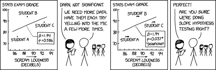
The (silly) graphs in the first and third panels of this comic show a (comically-) exaggerated example of dependent data. Notice that in the third panel, there are nine data points instead of three, but there is essentially no new information in the graph, compared to the first panel, because the new data points are strongly correlated with the original data points. The joke is that the female stick finger is ignoring this fact, conducting her second hypothesis test as if she really has a sample size of nine—in contrast, the male stick finger seems to intuit that the effective sample size has not changed. The point is that getting more data doesn’t always mean getting more information!
Avoiding Sticky Data
Whenever collecting sticky data, always ask yourself: What possible connections exist between each data point and the other data I’m collecting? In what ways do the data points have similar origins that reduce the data independence? What practical steps might I take that would increase the data independence? Try to avoid data that clump together because of similar origins and, if possible, randomize sequences of events.
Mantra
Avoid repeated sampling from the same source, related sources, or sources that can influence each other. These are sources of data dependence.