19 Relating Variables
(Modified on 2026-08-11)
1,725 words
In scientific inquiries we observe correlations between two or more “variables” that interest us. Generally, our goal is to describe, or better yet explain, the correlations between these variables. We will do this in prose, and this is often the most important part of our description. However, we will also use mathematical formulae and graphs to visualize relationships between variables.
In mathematical equations, we will often refer to independent variables as \(X_n\), with subscripts to differentiate multiple independent variables (\(X_1\), \(X_2\), etc.). In turn, dependent variables will be labeled \(Y_n\), though there is usually only one dependent variable, so it is simply \(Y\). As you might guess, we will typically visualize IVs on the \(X\) axis of graphs and dependent variables on the \(Y\) axis. This usage of \(X\) and \(Y\) will frequently be used even for non-experimental work: \(X\) might be a “predictor” variable and \(Y\) a “predicted” variable. However, when the relationship between \(X\) and \(Y\) is purely correlational, which one is \(X\) and which is \(Y\) is totally arbitrary.
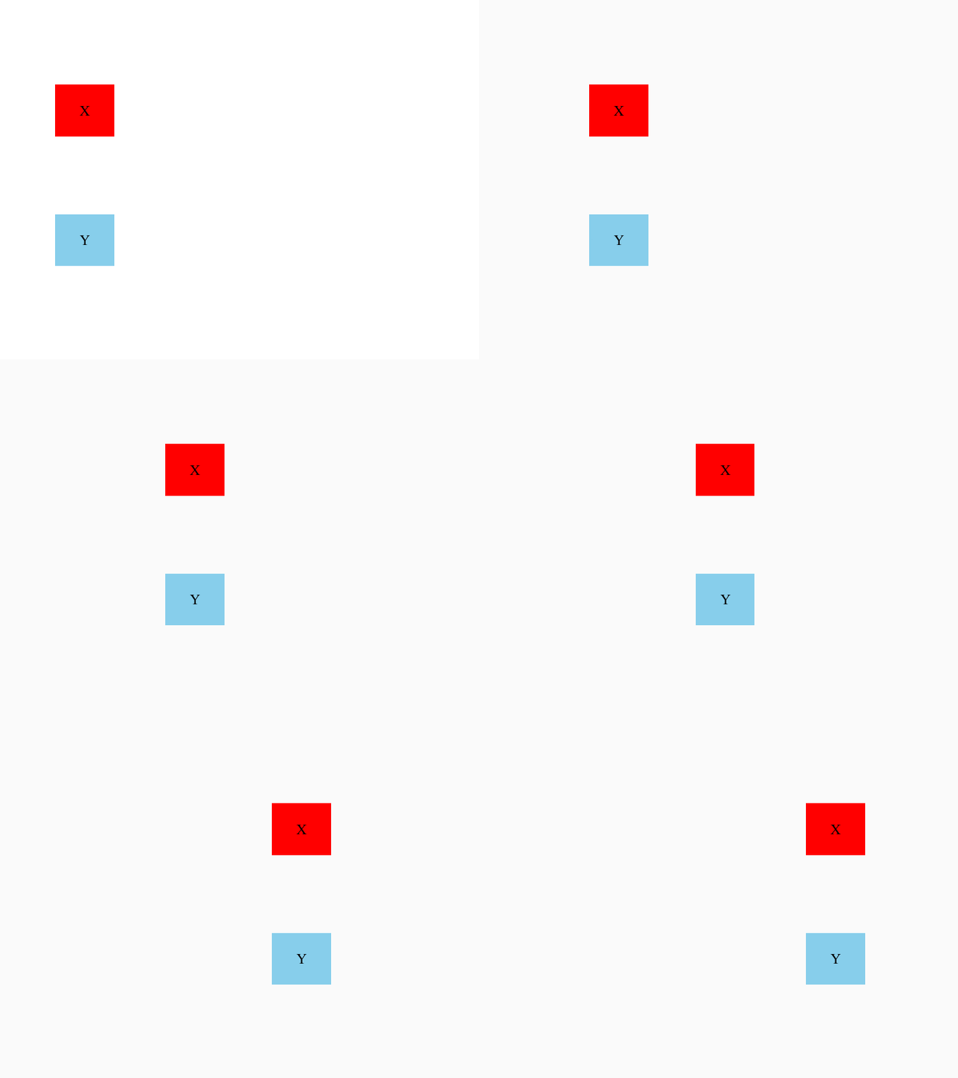
Correlation is, as we’ve discussed, an observed tendency for variation in one variable to be associated with changes in another variable. Note that “covariation” is commonly used as a synonym for correlation (though they have slightly different meanings in statistics). So for example, here the movement of the X and Y boxes are correlated:
If we measured the position of X and Y, and graphed them, we might see something like this:
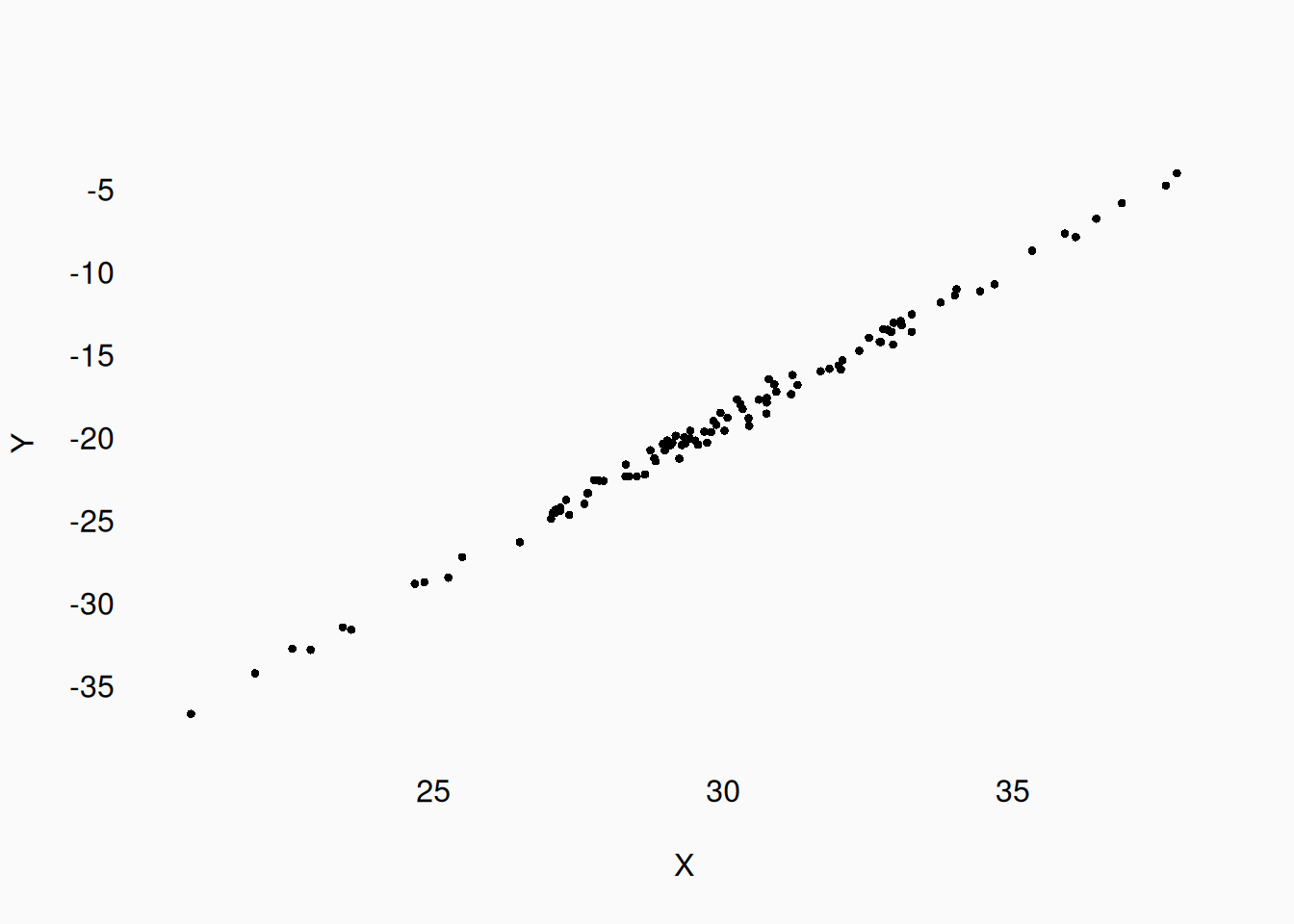
Now, “associated” can mean many things. For example, there can be a reversed or negative correlation:
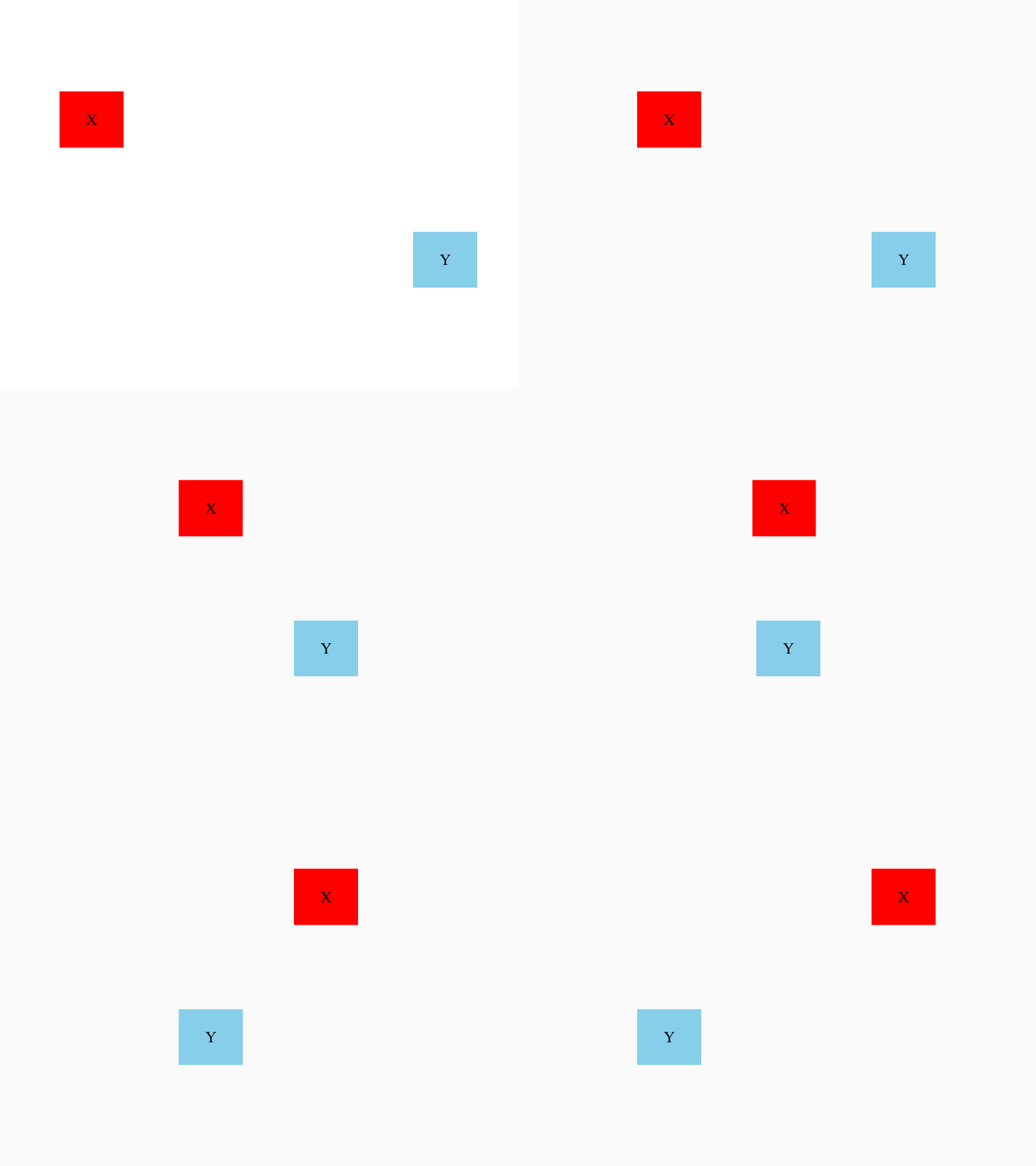
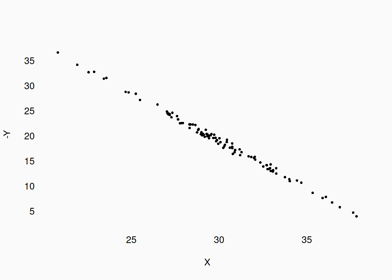
The correlation of these two variables is just as strong as in the previous example, but reversed. We might also observe correlations like this:
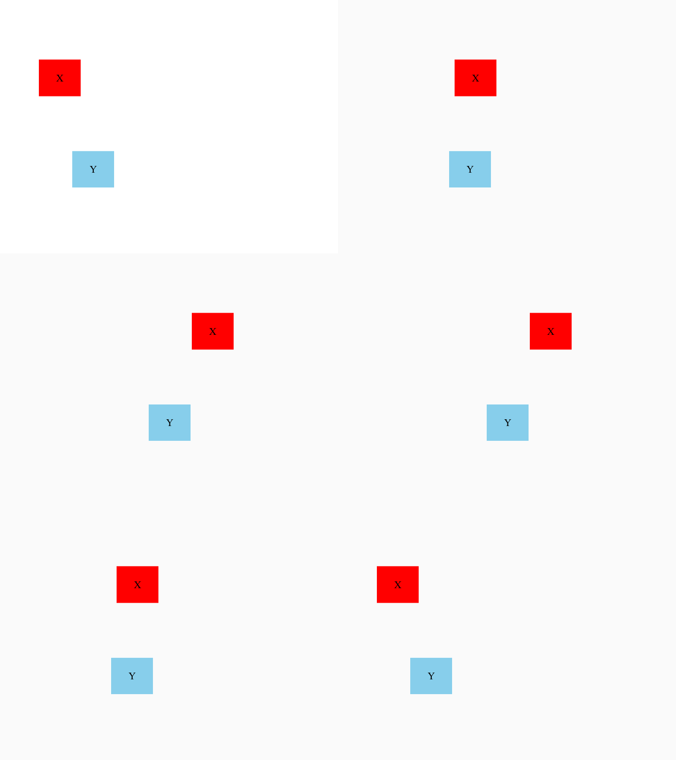
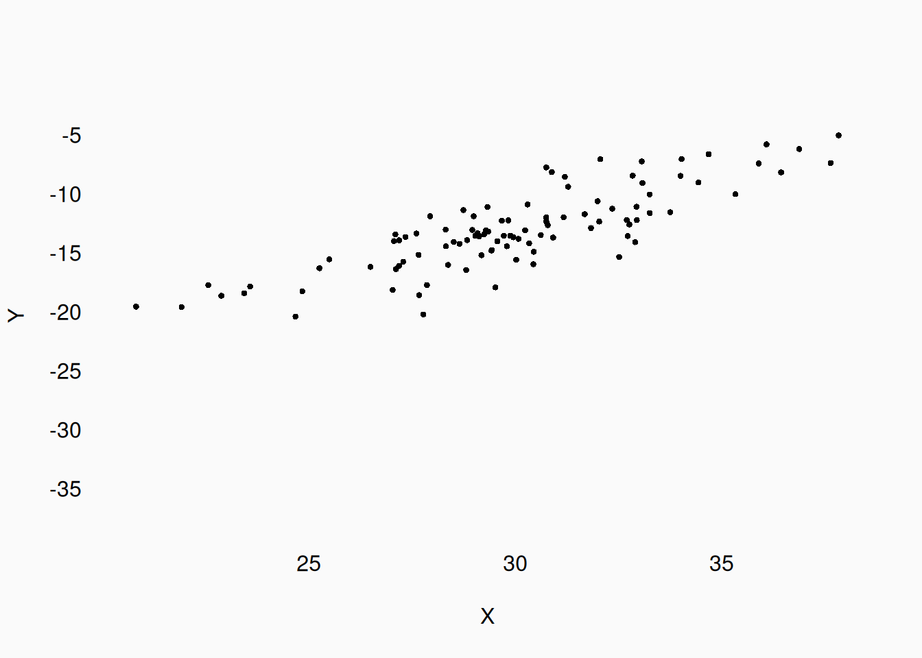
They still correlate, but the correlation is weaker.
Where do correlations come from? One possibility is that changes in one variable are causing changes in the other. Something like this, with X pushing Y:
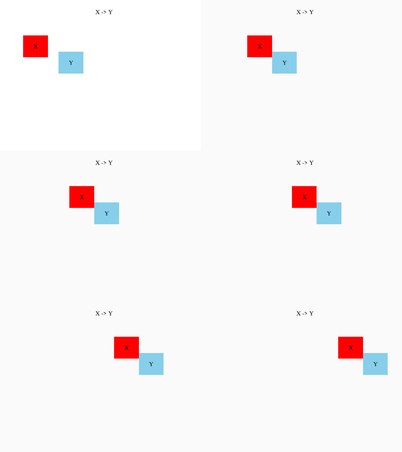
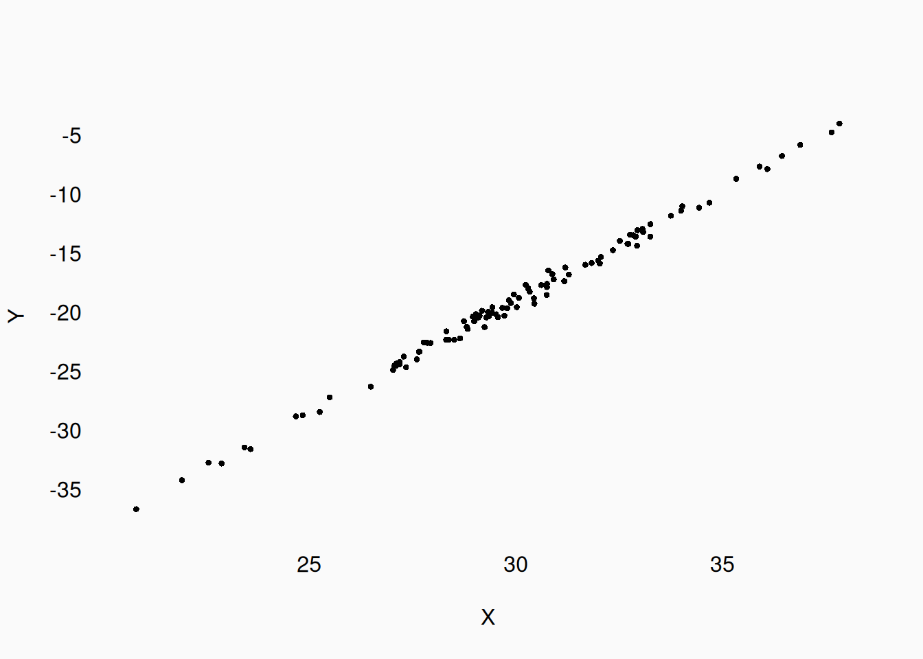
Notice that “causation” is not visualized in the graph—we only visualize the correlation! How would we know that X is causing (pushing) Y, and not being pulled by Y? We could manipulate X and see if Y changes. If Y is the one “pulling” X, then manipulating X shouldn’t affect Y.
Another possible explanation for an observed correlation is a third variable, which may be unobserved, affecting both variables.
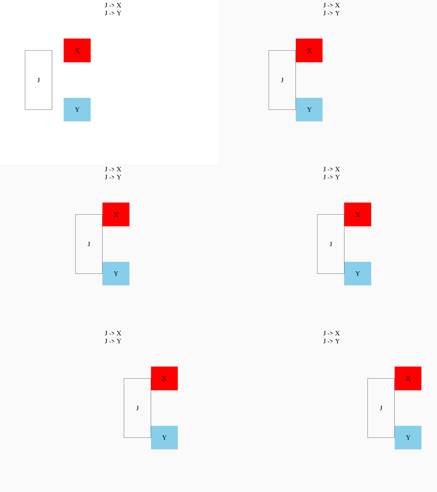
If we didn’t know about J, we’d never be able to explain the correlation between X and Y.
Direction
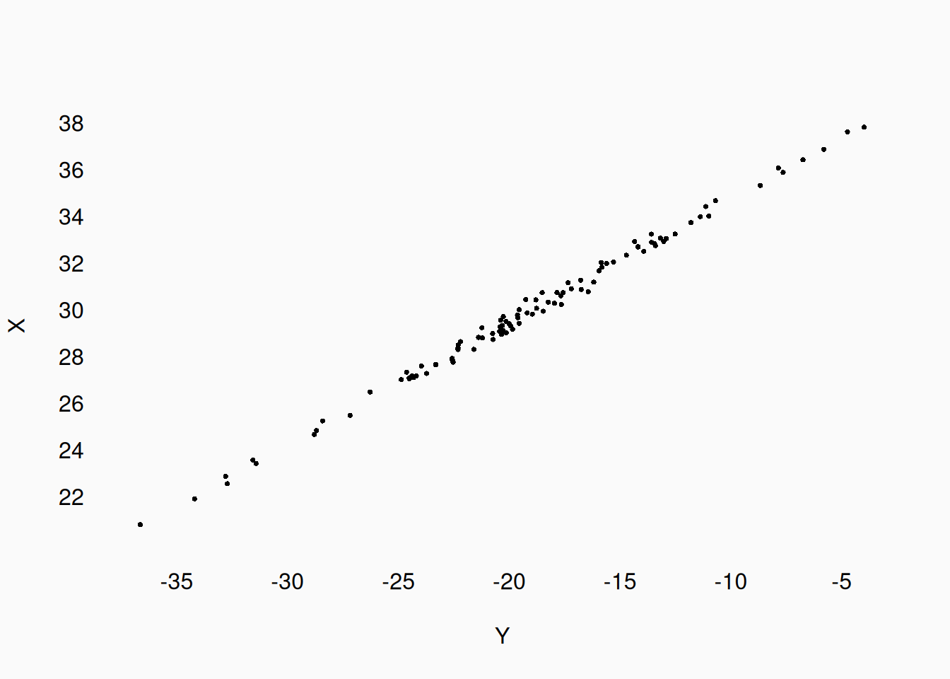
Correlation has no “direction.” We can only infer causal direction from other information (i.e., knowing that we manipulated something). In many correlational studies, one variable will be presented as the “predicted” or “dependent” variable, plotted on the Y-axis, while another variable is presented as the “predictor” or “independent” variable, plotted on the X-axis. However, without additional evidence about causation, we can always “flip” the plot/named direction between variables:
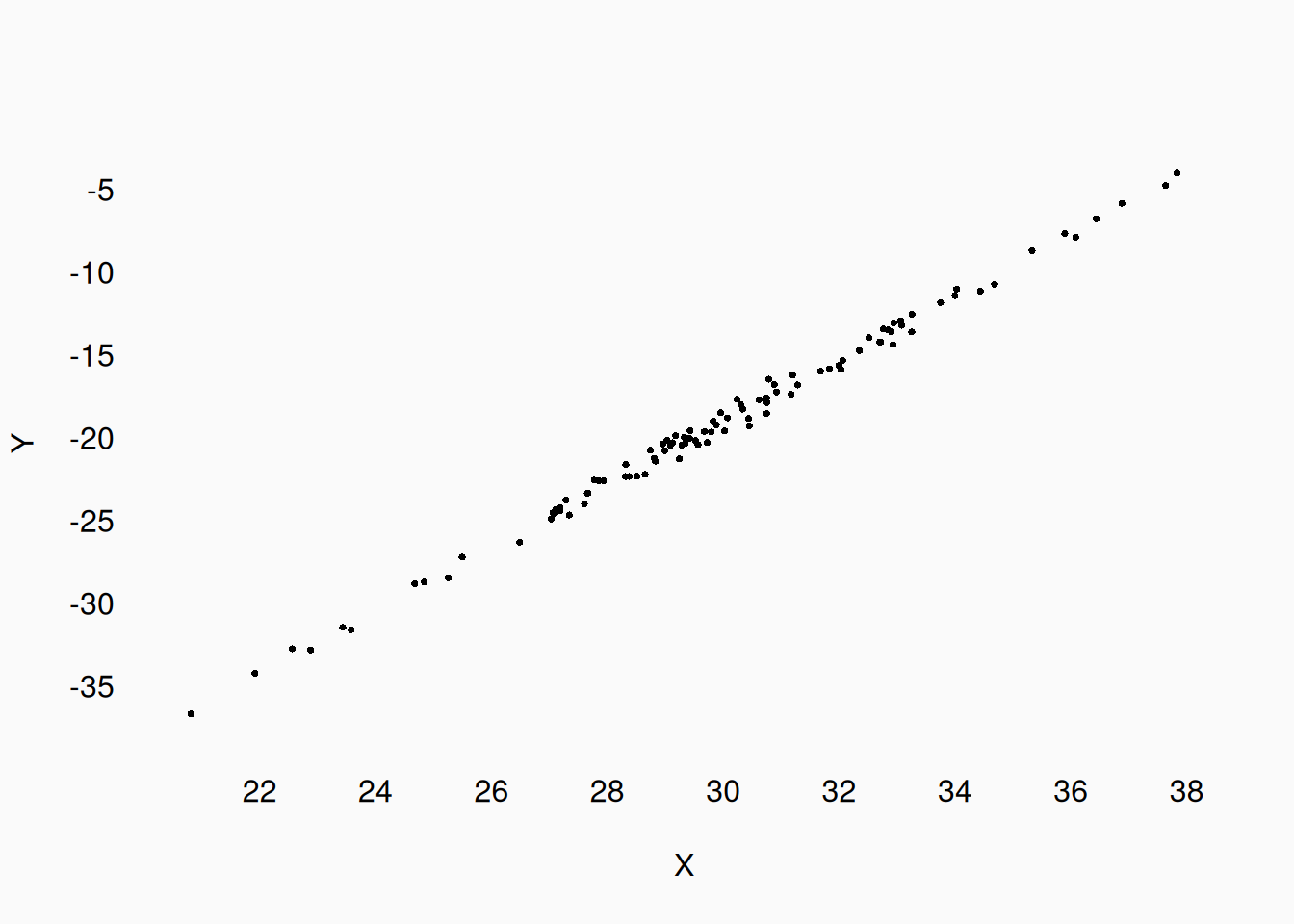
or…
Three-way correlations
We might observe three (or more) variables correlating, in one way or another. With more than two variables, other relationships become possible.
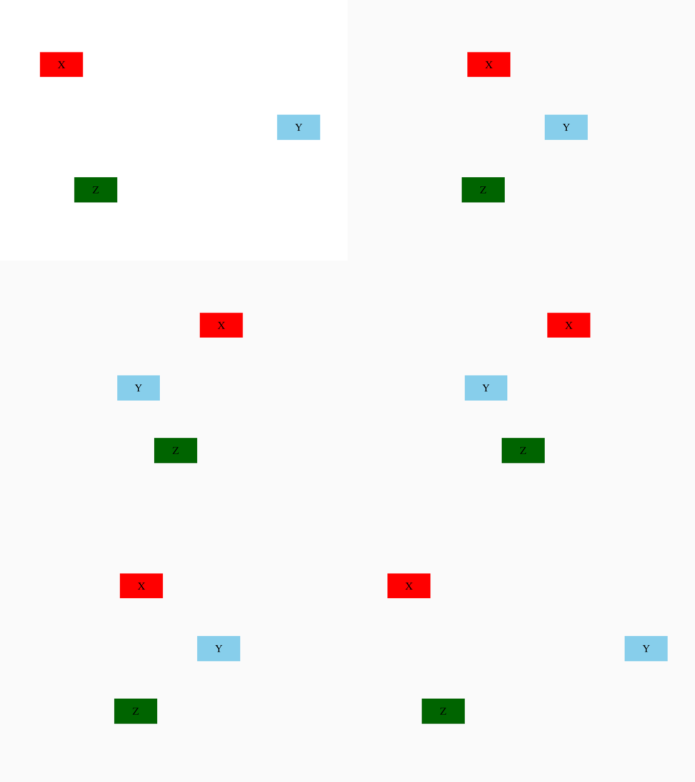
We can attempt to visualize this in three dimensions (examples below), but it is usually more effective to visualize the correlation between each pair of variables. With three variables, there are three pairs to visualize:
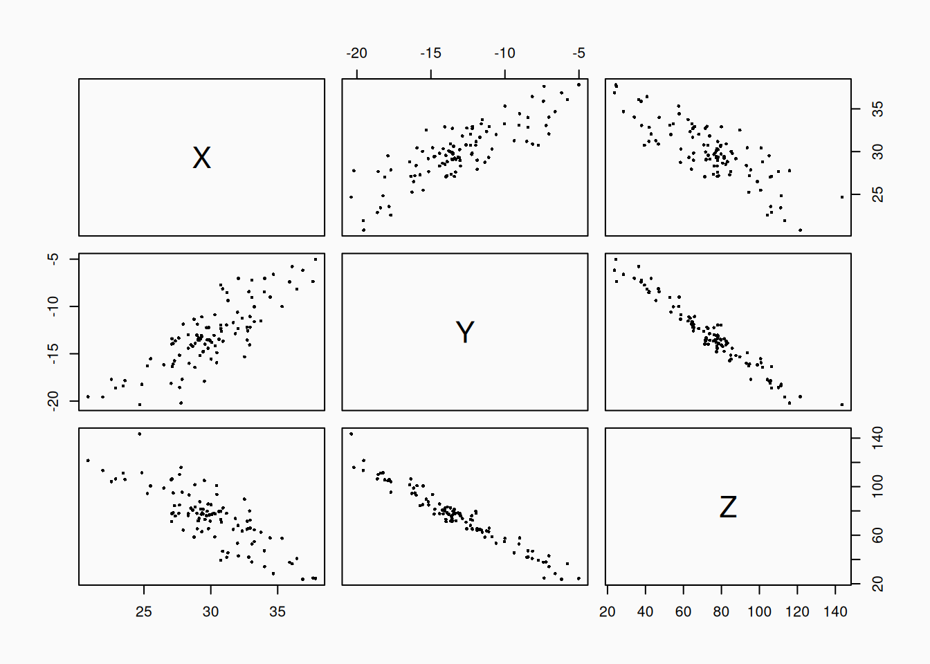
How might we explain three (or more) variables correlating? One possible explanation is a mediating relationship:
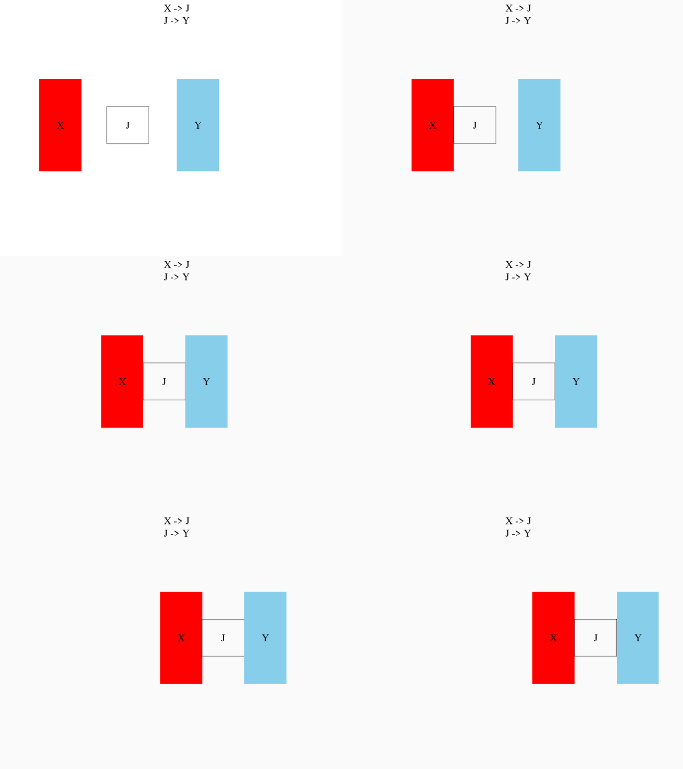
In mediation, \(X\) influences \(J\), which in turn influences \(Y\). In this case, \(J\) would be called a mediator variable. It can be very hard to distinguish mediation from “true” direct causation.
Recall the elevator music \(\rightarrow\) pro-social behavior from the scientific inquiry. If we play loud death metal music in an elevator, many people might simply react by covering their ears. Walking out of the elevator with their hands on their ears, they might be less likely to notice somebody dropping their books on the ground, and thus, be less likely to stop and help. In this case, it may be the mediating variable (ears covered vs uncovered) which affects pro-social behavior, not the music itself. Of course, we might still conclude that playing death metal in the elevator (indirectly) reduces pro-social behavior, but our understanding of what is really happening is clouded if we fail to identify the mediating variable.
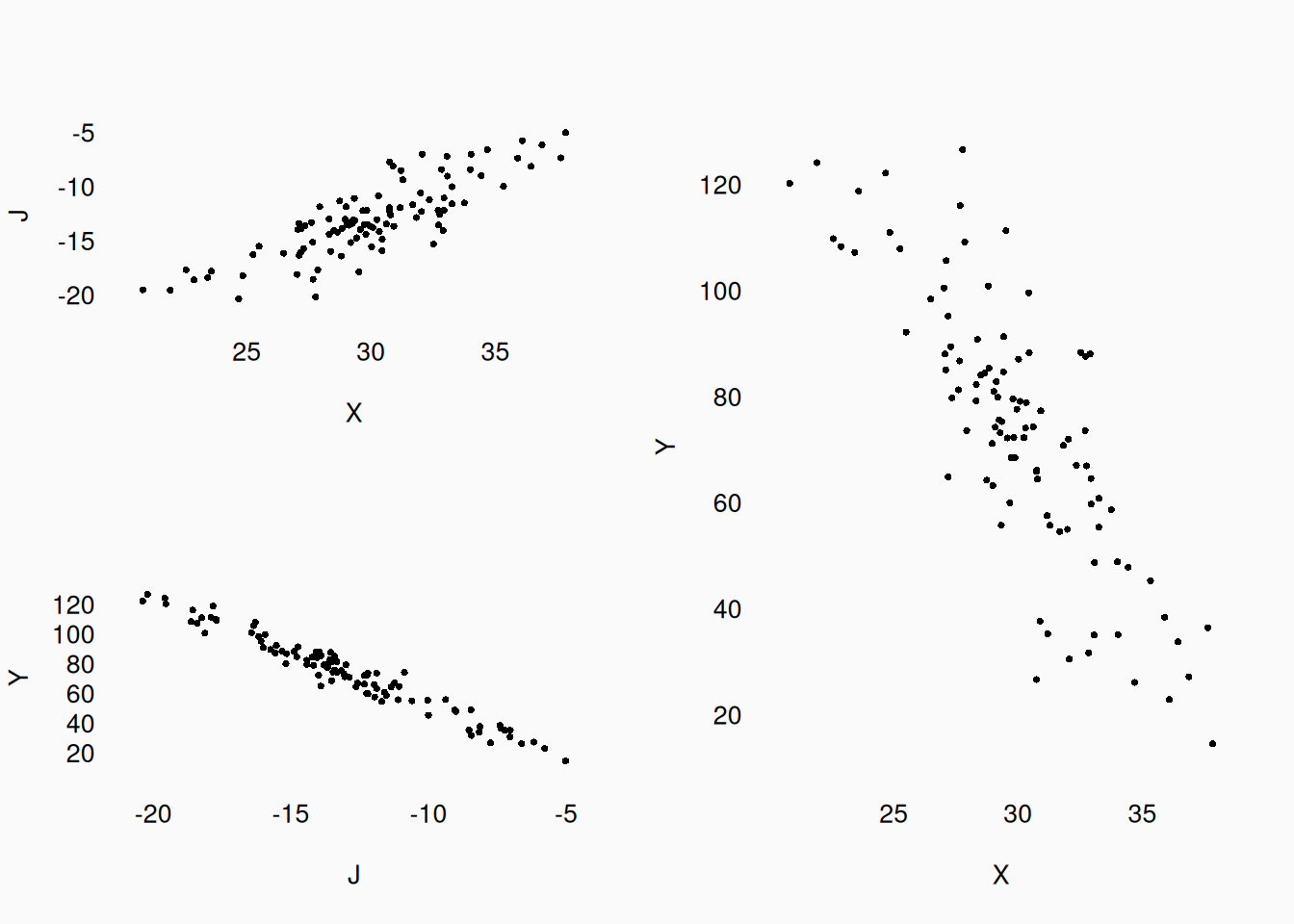
The following graph shows data for three variables, generated with a mediation relationship. \(X\) and \(Y\) are not actually directly related—they are only related through the mediator \(J\). But if you just look at the plot of \(X\) vs \(Y\), there’s no way to tell that! If we didn’t know about \(J\), we could easily be convinced that \(X\) influences \(Y\).
Multiple independent variables
In many studies, there will be multiple independent variables influencing (or at least predicting) a dependent variable. Each variable’s independent effect is called its main effect.
In the simplest case, the effect of the IVs is independent; when taken together, their effects are simply added together. In an equation, we’d write something like \(X_1 + X_2 = Y\), where \(X_1\) and \(X_2\) are independent variables, and \(Y\) is the dependent variable. For example, consider this demonstration:
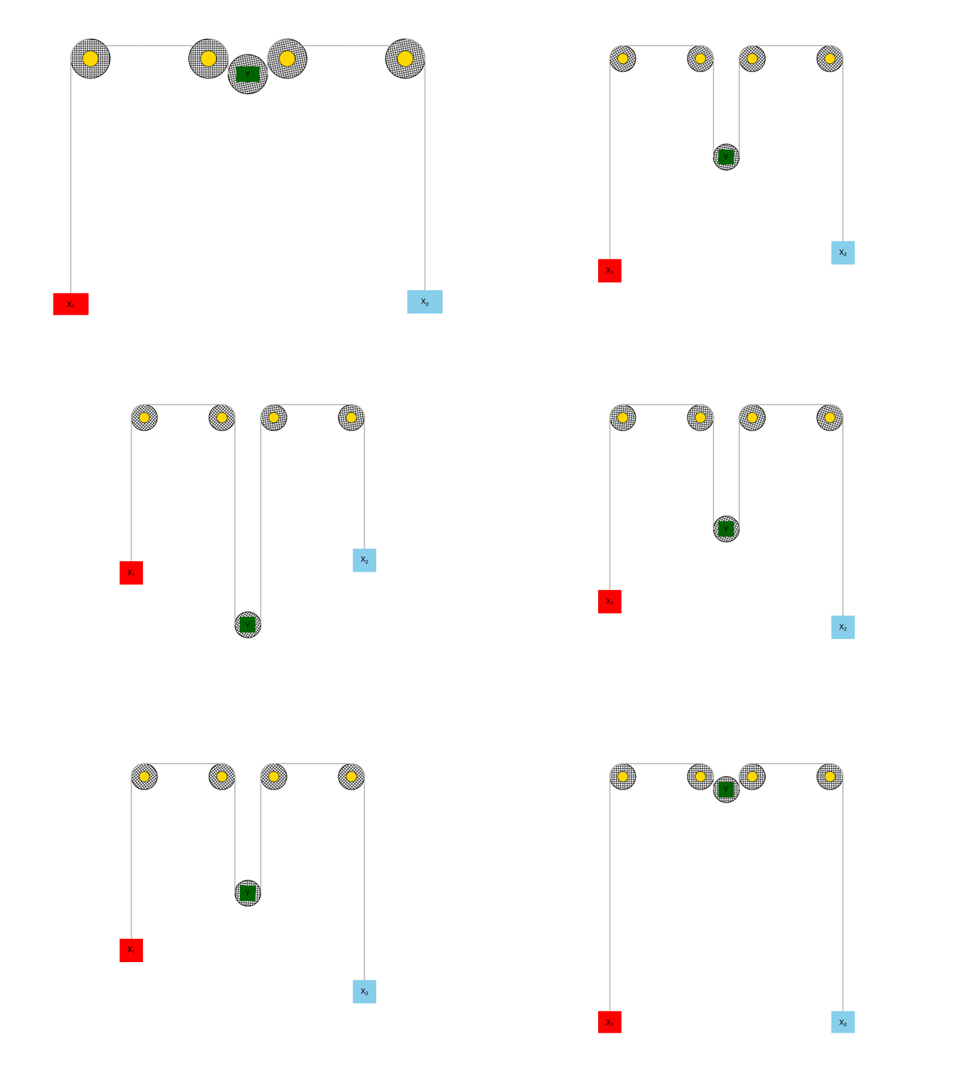
Here, because they are connected using pulleys, our \(X_1\) and \(X_2\) variables are both negatively correlated with \(Y\). Raising \(X_1\) or \(X_2\) each independently causes \(Y\) to lower, and this effect is the same regardless what the other \(X\) is doing. However, their two effects are added together: if both \(X_1\) and \(X_2\) rise, \(Y\) drops faster; if \(X_1\) rises while \(X_2\) drops, their effects cancel out and \(Y\) stays still.
In a plot, if our main effects are independent, then individual scatter plots between \(Y\) and each variable look just like any other correlational plot:
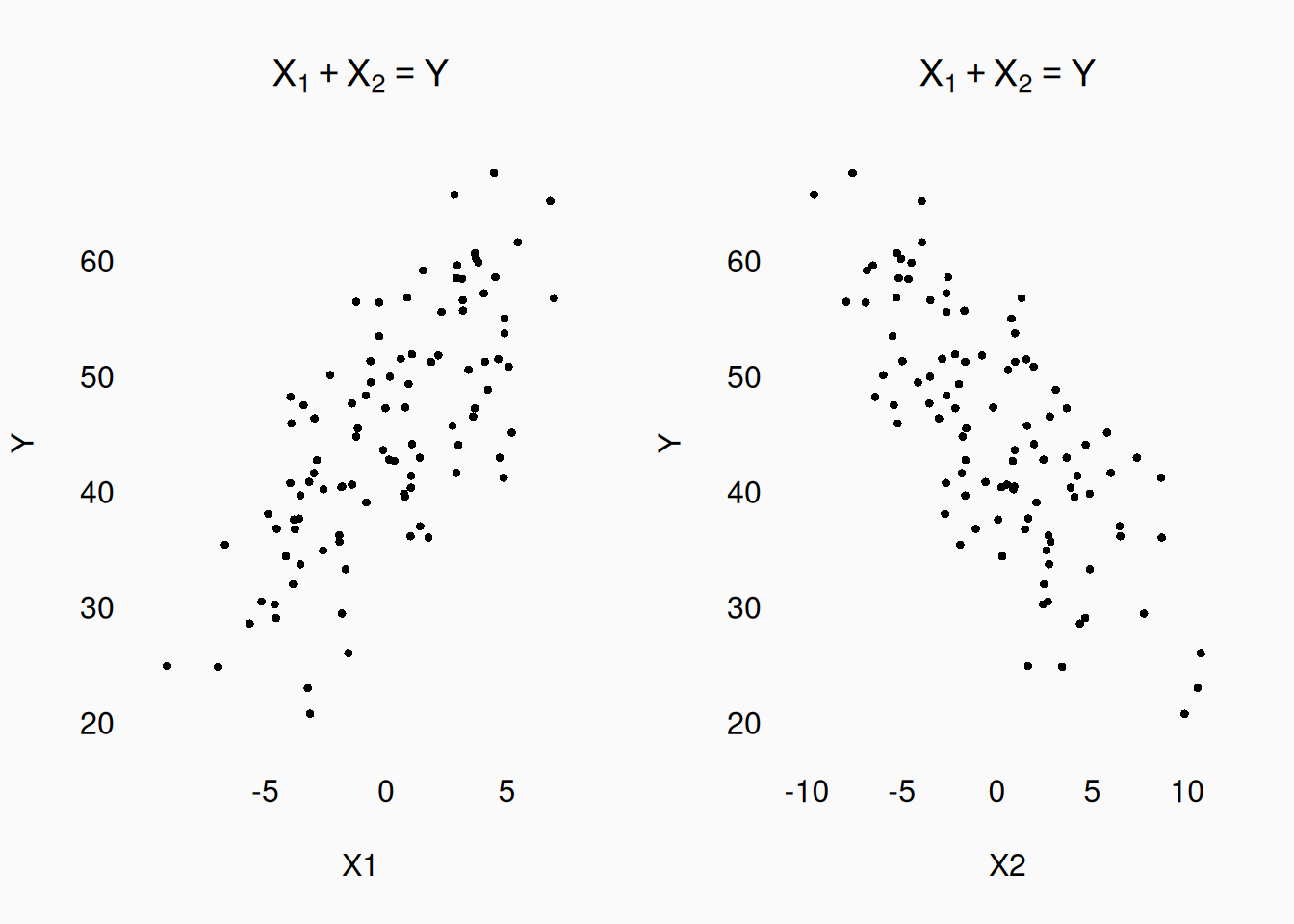
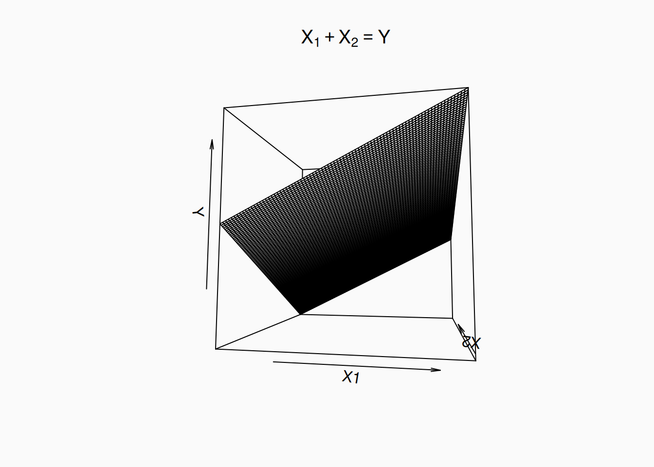
If we try to visualize all three variables in a single, 3D plt, this sort of independent, “summing” relationship will look like a flat plane:
A possible example of additive effects in music might be the influence of tempo and timbral “brightness” on the expression of happiness. We’d expect to see a positive correlation between musical tempo and the perceived happiness of the music; we’d also expect there to be a positive correlation between timbral “brightness” and perceived happiness. To test these predictions, we could do an experiment. We could create musical stimuli where we manipulate each of these variables into three levels, creating a factorial \(3 \times 3\) design with 9 total conditions (nine pieces of musical stimuli). We could then have ten people listen to each of our stimuli and rate how happy they found each one.
| Slow tempo | Moderate tempo | Fast tempo | |
|---|---|---|---|
| Dark timbre | \(N = 10\) | \(N = 10\) | \(N = 10\) |
| Moderate timbre | \(N = 10\) | \(N = 10\) | \(N = 10\) |
| Bright timbre | \(N = 10\) | \(N = 10\) | \(N = 10\) |
If we calculate the mean happiness rating in each of our nine conditions, we’d expect to see something like this:
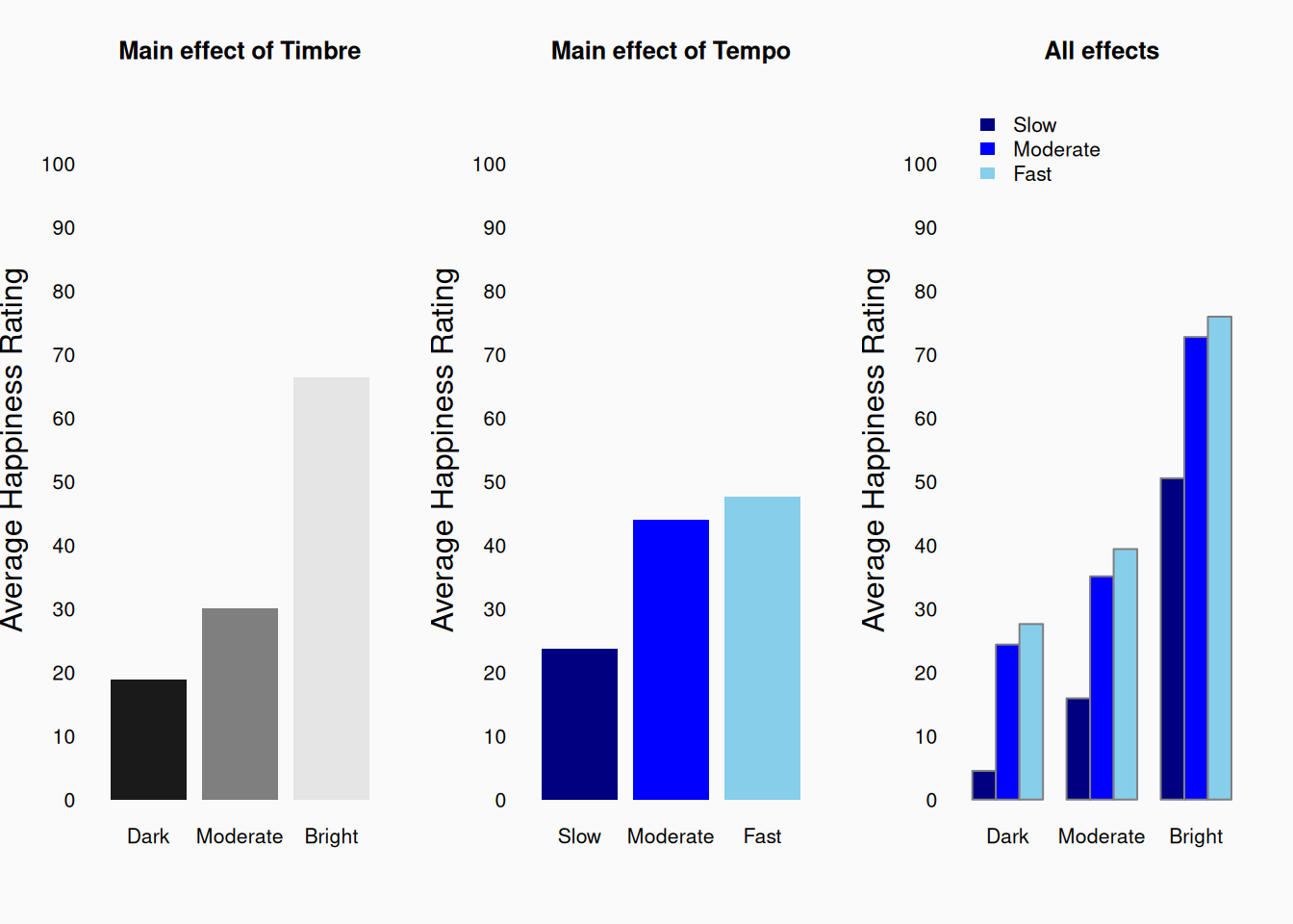
The left two figures above are showing the independent main effects of timbre and tempo independently. In other words, I’ve averaged ratings across the three levels of each variable while ignoring the other variable. It’s easy to see that both variables have a positive main effect on happiness ratings.
The rightmost figure above is showing the average rating for each of the nine conditions. In this graph, we can see that the two effects sum together: when the tempo is fast and the timbre is bright, we get the maximally happy music; When the tempo is slow and the timbre is dull, we get the minimally happy music. We can also see that for example, a dark timbre cancels out a fast tempo (to some extent). Indeed, this graph illustrates a purely “additive” relationship, meaning that tempo always has the same effect regardless of timbre, and vice versa. Fast dull sounds are happier than slow dull sounds; fast bright sounds are happier than slow bright sounds. The two effects are totally independent of each other. These specific differences of effects within the level of another variable are called simple effects.
Interactions
When working with two or more independent variables, there is another important possibility to consider. Changes in two (or more) variables may interact when influencing a third. This means that the influence of \(X_1\) on \(Y\) depends on the value of \(X_2\).
This graphic illustrates an interactive relationship involving a lever:
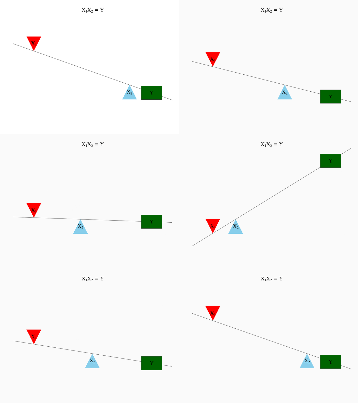
Here, changes in \(X_1\) and \(X_2\) both affect \(Y\), but the effect depends on what the other \(X\) is doing. For example, when \(X_2\) is far to the left, \(X_1\) has a strong negative effect on \(Y\); however, when \(X_2\) is far to the right, \(X_1\) has a weak positive effect on \(Y\).
Mathematically, an interaction between effects is represented by multiplication: \(X_1 * X_2 = Y\). To fully describe the relationship between \(X_1\), \(X_2\), and \(Y\) above, we need a more complicated equation like
\[ X_1 + X_2 + X_1 * X_2 = Y \]
In this equation,
- \(X_1\) is the main effect of \(X_1\)
- \(X_2\) is the main effect of \(X_2\)
- \(X_1 * X_2\) is the interaction between \(X_1\) and \(X_2\)
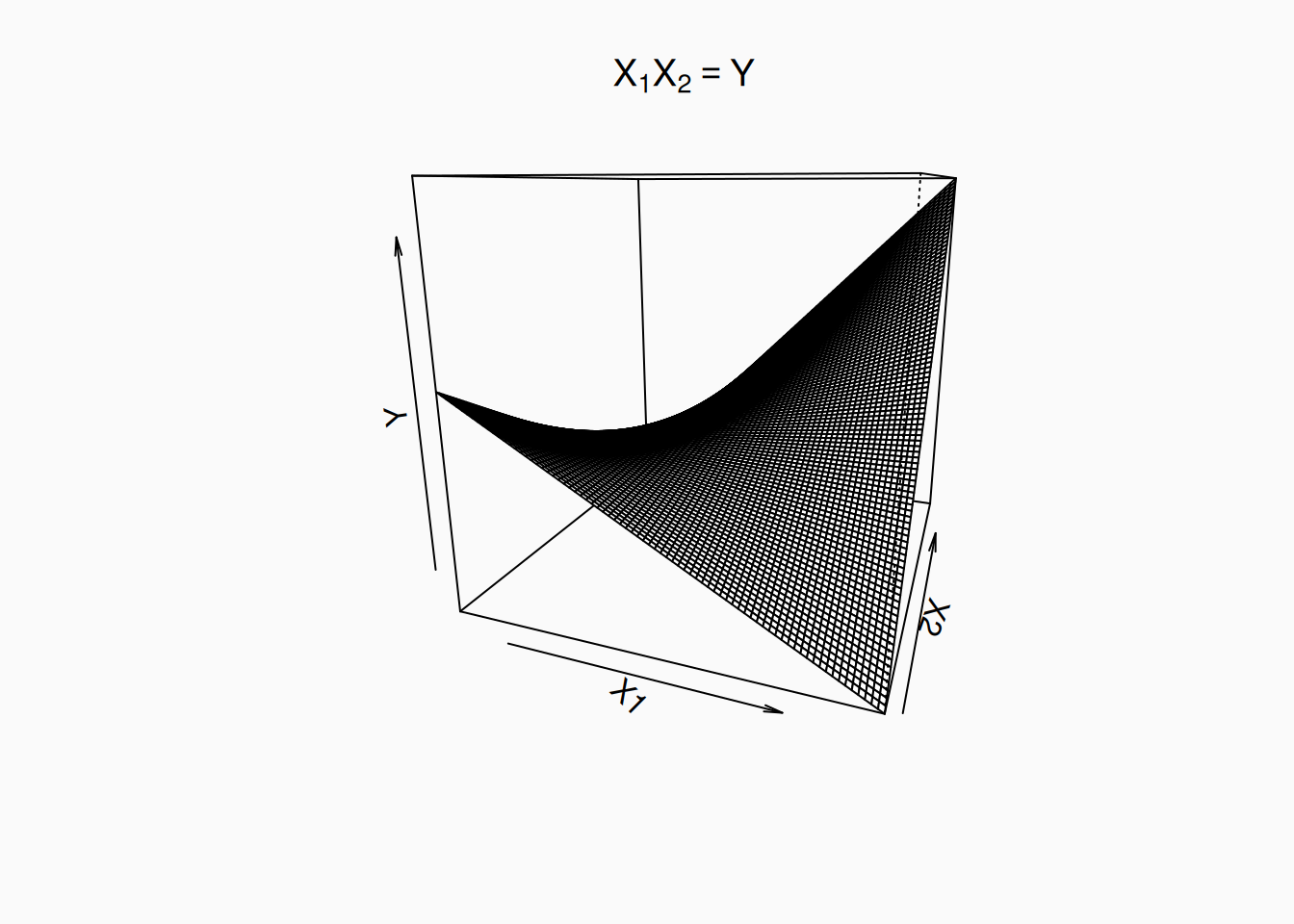
If we visualize an interaction in three continuous dimensions, we’ll see a curved surface:
As a possible example of interactive effects in music research, lets think about the effects of tempo and mode (major vs minor) on perceived happiness. Generally, we predict major to elicit happier responses than minor. However, at a very high tempo, the minor mode might start to sound less sad and more heroic, nervous, or angry—not happy. Conversely, at a slow tempo, minor might start to sound peaceful and/or relaxing—which are happy feelings. Thus, we encounter a situation where the effect of one variable depends on the level of the other variable. If we conducted a similar experiment to our timbre/tempo experiment, we might see graphs like these:
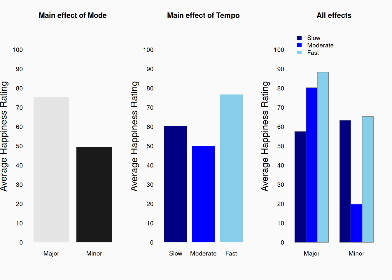
Again, our two left graphs show the (independent) main effects, which match what we’d expect. But if we look at the plot of all nine conditions we can see that there is more going on here. If we look at the simple effect of mode when the tempo is slow, we see that minor music made responses (slightly) more happy! We can also see that the difference between major and minor music is smaller for fast tempos than it is for moderate tempos.
These sorts of “interactions” happen all the time. In fact, in psychology research, hypotheses are often about interactions. In order to measure interactions, we need to measure all relevant variables, and “cross” all their levels in full factorial designs.
Beyond three dimensions
When the numbers of variables increase, the number of possible additive, interactive, or mediative relationship possibilities explodes! If we have, for example, ten variables, there are 45 two-way relationships, 120 three-way relationships, 210 four-way relationships, etc. And of course, there may also be missing, unknown variables which we haven’t measured. In these situations, it can be very difficult to determine what true relationships exist in our data. This is part of the challenge (and the risk) of exploratory research—trying to look at a bunch of correlations and come up with theoretical explanations is hard. Conversely, this is part of why a priori predicted relationships are important! We go into an analysis knowing what we are looking for.