1:	☼ ○ ☼ ○ ☼ ○ ♣ ♥ ○ ♣ ♥ ☼ ○
2:	♠ ♥ ♠ ♥ ♠ ♥ ♠ ♥ ○ ♦ ♥ ○ ♦ ♥ ○ ♦ ♠ ♥
3:	♠ ♥ ○ ♦ ♥ ♠ ♥ ♠ ♥ ♠ ♥ ♠ ♥ ♠ ♥ ♠ ♥ ○ ♦
4:	♠ ♥ ♠ ♥ ♠ ♥ ♠ ♥ ○ ♦ ♥ ○ ♦ ♥
5:	♣ ♦ ♣ ♦ ♥ § ♦ ♣ ♦ ♥ § ♦ ♣ ♦
6:	☼ ○ ☼ ○ ♣ ♥ ○ ☼ ○ ☼ ○ ☼ ○ ☼ ○ ☼ ○ ☼ ○
7:	♠ ♥ ♠ ♥ ♠ ♥ ♠ ♥ ♠ ♥ ♠ ♥ ○ ♦
8:	♦ ♠ ♦ ♠ ☼ ♣ ♠ ♦ ♠ ♦ ♠ ☼ ♣ ♦ ♠ ♦ ♠ ☼
9:	♦ ♠ ☼ ♣ ♠ ♦ ♠ ☼ ♣ ♠ ☼ ♣ ♠ ♦ ♠ ♦ ♠ ♦
10:	♥ ☼ § ♠ ☼ ♥ ☼ § ♠ ☼ ♥ ☼ ♥ ☼ ♥ ☼ § ♠ ☼
11:	☼ ○ ☼ ○ ♣ ♥ ○ ♣ ♥ ○ ☼ ○ ☼ ○ ☼ ○ ☼ ○ ♣
12:	♣ ♦ ♥ § ♦ ♣ ♦ ♣ ♦ ♥ § ♦ ♣ ♦ ♣ ♦ ♣ ♦
13:	♥ ☼ ♥ ☼ ♥ ☼ ♥ ☼ § ♠ ☼ ♥ ☼ ♥ ☼
14:	☼ ○ ☼ ○ ☼ ○ ☼ ○ ♣ ♥ ○ ☼ ○ ♣ ♥ ○
15:	♦ ♠ ♦ ♠ ♦ ♠ ♦ ♠ ♦ ♠ ♦ ♠ ♦ ♠
16: ☼ ○ ☼ ○ ♣ ♥ ○ ♣ ♥ ☼ ○ ☼ ○ ☼ ○ ☼40 Encoding Music
(Modified on 2026-08-11)
6,128 words
All musical performances (including mechanical playback of recordings) consist of continuous sound signals: that is, extremely tiny and rapid fluctuations of air pressure over time. We can encode this sound very faithfully by measuring these fluctuations 44,100 times per second on a integer scale with \(2^{16}\) levels. That’s 705,600 bits of information per second! However, musical sound signals are highly organized, including lots of redundancy and repetition. This organization is not obviously apparent in the “raw” signal—it requires processing and modeling to understand, and appreciate, it.
The cognition of musical organization involves many mental processes, from low-level perceptual processes like pitch perception, auditory scene analysis, and event binding, to high-level processes like anticipation, autobiographical recall, and social/emotional appraisal. The point is that a musical (sound) signal has a lot of information in it, but extracting and understanding that information is not simple.
Musical pieces and performances are complex, multi-dimensional constructs. We, as musicians and listeners, use both conscious and unconscious (intuitive) mental models to understand those constructs. Some ways in which we model music include:
- As orthogonal dimensions:
- Musical sounds can be modeled in terms of several more-or-less orthogonal dimensions—pitch, rhythm, dynamics, timbre, lyrics, etc.
- As discrete events:
- The continuous stream of musical sound can be modeled as a series of discrete musical events—most fundamentally, “notes.” Notes are “events” that start (onset) and end (offset) at particular times, and typically have properties like pitch and timbre.
- As hierarchical structures:
- Note events are arranged and grouped in hierarchically nested “structures,” like motives, phrases, and sections.
- As pitch structures:
- Continuous frequency space is divided into discrete pitch categories, which are organized into scales and other hierarchical structures.
- As temporal structures:
- The timing of musical events is highly organized, usually in relation to isochronous pulses—beats.
I emphasize that these are all models of music, and as we know, All models are wrong, but some are less wrong. None of these models are “objectively real”; However, they can be useful. Creating and studying models of music is the domain of music theory. Some music theories are etic—consciously used or discussed by musicians and listeners themselves; Other theories are emic—discussed by academics, but not used (consciously) by musicians. In engineering, knowledge about musical structures is an example of “domain knowledge.”
Encoding Musical Knowledge
A digital audio recording can serve as a faithful representation of “raw” sound, good enough to reproduce the sound with little or no perceivable difference from the original sound. However, this representation is not (directly) useful for many other purposes. In contrast, more abstract, theory-driven representations of musical structures and objects can be very useful, because they reflect (or embed) domain knowledge. A formalized system for representing theoretical musical objects—especially lower-level objects like “notes”—is an encoding scheme. Labels of higher-level information about musical structures are called annotations, especially when they are added to or aligned with “score-like” note data. Examples of annotations include phrases/grouping markers, formal analyses, and chord labels.
Note: Music theory models are not the only useful models of the information contained in audio recordings. For example, there are many acoustical models that can be used to model or characterize musical performances in useful ways. These are usually called audio “features” and we will discuss them in the next chapter.
Layers of meaning
Good news! An ethnomusicologist colleague of yours has just returned from a remote part of Indonesia, where they have been doing field work studying the music of a local society. While in the field, they transcribed some of the musical performances they witnessed, and now they are giving the transcriptions to you to analyze! Hooray!
Their transcriptions use symbols drawn from that society’s musical vernacular; These symbols essentially represent instructions for which notes to play on a specific local instrument. Here are some of the transcriptions (one per line, read left to right):
Odd looking scores to us, but perhaps meaningful to the people of that culture.
If we inspect these transcriptions closely, we can discover some patterns. For example, the symbol ☼ frequently transitions to ○, while ♠ never does. Perhaps with more analysis, we could learn more about this culture’s music. However, it would be helpful to know more about the symbols—for now, all we know is that the transcription represents a categorical variable with seven levels.
Fortunately, your ethnomusicologist colleague brought one of these instruments home with them, and they show you how to play each symbol on the instrument. You are able to play each of the seven symbols and measure their resulting pitch, and you find that they are approximately equivalent to a just-intonation major scale. Based on this, you are able to translate their encodings to a more familiar (approximate) equivalent:
1:	E B E B E B C A B C A E B
2:	D A D A D A D A B G A B G A B G D A
3:	D A B G A D A D A D A D A D A D A B G
4:	D A D A D A D A B G A B G A
5:	C G C G A F G C G A F G C G
6:	E B E B C A B E B E B E B E B E B E B
7:	D A D A D A D A D A D A B G
8:	G D G D E C D G D G D E C G D G D E
9:	G D E C D G D E C D E C D G D G D G
10:	A E F D E A E F D E A E A E A E F D E
11:	E B E B C A B C A B E B E B E B E B C
12:	C G A F G C G C G A F G C G C G C G
13:	A E A E A E A E F D E A E A E
14:	E B E B E B E B C A B E B C A B
15:	G D G D G D G D G D G D G D
16:	E B E B C A B C A E B E B E B E
These symbols are more familiar to us, which makes this easier to read. But we have also gained something much more important: we have additional knowledge about the structure of this variable. Notably, we know that these symbols have an order, which allows us to see additional patterns that we couldn’t before. For example, we can now recognize that every piece begins with the same perfect fifth interval: A-E, C-G, E-B, G-D, or D-A.
Excited by this discovery, you call up your ethnomusicologist colleague and tell them about it. They respond:
Well that makes sense! In their music tradition, the first note of the piece is considered the “home” note, and all other notes follow from it.
That description, of course, sounds a lot like the “tonic” note of Western music. You might wonder, why couldn’t we have just written down the transcriptions that way in the first place? For example, if we made the “home” note “1,” and numbered all the other notes relative to that first step? The result would look like this:
1:	1 5 1 5 1 5 6 4 5 6 4 1 5
2:	1 5 1 5 1 5 1 5 6 4 5 6 4 5 6 4 1 5
3:	1 5 6 4 5 1 5 1 5 1 5 1 5 1 5 1 5 6 4
4:	1 5 1 5 1 5 1 5 6 4 5 6 4 5
5:	1 5 1 5 6 4 5 1 5 6 4 5 1 5
6:	1 5 1 5 6 4 5 1 5 1 5 1 5 1 5 1 5 1 5
7:	1 5 1 5 1 5 1 5 1 5 1 5 6 4
8:	1 5 1 5 6 4 5 1 5 1 5 6 4 1 5 1 5 6
9:	1 5 6 4 5 1 5 6 4 5 6 4 5 1 5 1 5 1
10:	1 5 6 4 5 1 5 6 4 5 1 5 1 5 1 5 6 4 5
11:	1 5 1 5 6 4 5 6 4 5 1 5 1 5 1 5 1 5 6
12:	1 5 6 4 5 1 5 1 5 6 4 5 1 5 1 5 1 5
13:	1 5 1 5 1 5 1 5 6 4 5 1 5 1 5
14:	1 5 1 5 1 5 1 5 6 4 5 1 5 6 4 5
15:	1 5 1 5 1 5 1 5 1 5 1 5 1 5
16:	1 5 1 5 6 4 5 6 4 1 5 1 5 1 5 1
If we inspect this data, what more can we see? Well, for one, there are only ever four notes used in any piece: 1, 4, 5 and 6. What’s more, there are only 6 note transitions that ever occur in the data!
1 -> 5
4 -> 1
4 -> 5
5 -> 1
5 -> 6
6 -> 4
We have now considered three different encodings of the same data:
- ☼ ○ ☼ ○ ☼ ○ ♣ ♥ ○ ♣ ♥ ☼ ○
- E B E B E B C A B C A E B
- 1 5 1 5 1 5 6 4 5 6 4 1 5
From top to bottom, these representations move from more specific and “raw” to more abstract and theoretical. The original notation contains the most “raw” information—it simply indicates which note is played on a specific type of instrument. The more abstract representations, however, embed more domain knowledge into each symbol, by assuming and superimposing theoretical models on the information: scale order and tonal-center respectively. Our ethnomusicologist friend was aware, from the beginning, of the scale-order and tonal-centeredness of the music, but this information was not in the transcriptions. We had to interpret the data using our understanding of order and tonal center. By superimposing a model (knowledge) onto the data, we are able to make more inferences.
When we embed assumptions into our encodings, we pack more information into each symbol, but risk misunderstanding the data.
By interpreting the symbols we are also making more assumptions about the symbols. For example, we assumed that because the notes are close to what we call a major scale, it is appropriate to label them in order like C-D-E-F-G-A-B, as we would in Western music. Is this etic assumption reasonable? Maybe, maybe not. Could the emic view of this scale differ from ours in some important way?—Like perhaps they order them G-F-E-D-C-B-A-G? In our final, tonally-centered representation, we further assume that the absolute pitch doesn’t matter, only the relationships between scale steps. If we embed these assumptions, or assumptions like them, into our encodings, we pack more information into each symbol, but risk misunderstanding the data.
Qualitative and Quantitative Encoding
When we move from “♣” to “C” to “1,” each move embeds additional knowledge into the symbol, but also discards (potentially useful) details. The original representation is more qualitative—more complete, more raw, and making fewer assumptions. The later representations are more quantitative—more abstract, more dependent on modeling and assumptions, and easier to analyze. There are advantages and disadvantages either way. If your ethnomusicologist friend had started by giving you the final, numeric representation, you would have no way of studying the absolute pitch information. Similarly, if they had given you the letter-name representation, you wouldn’t have known what specific notes to play on the culture’s musical instrument. On the flip side, if you start with the “♣” symbols, there is no way for you to recognize more abstract patterns without applying outside knowledge to the data. For example, there would be no way to possibly infer that the sixth degree always transitions to the fourth degree.
The ethnomusicology example above illustrates that different aspects of musical domain knowledge can be included or omitted from encodings. We can observe the same thing strictly within conventional Western music theory and practice. For example, consider these four representations of the same melody:
    Hertz MIDI Scientific Degree  Lyric
1  261.39   60         C4      5    Hey
2  219.67   57         A3      3  Jude,
3  220.21   57         A3      3  don't
4  261.68   60         C4      5   make
5  293.86   62         D4      6     it
6  195.83   55         G3      2   bad.
7  195.87   55         G3      2   Take
8  220.17   57         A3      3      a
9  232.99   58        Bb3      4    sad
10 349.22   65         F4      1   song
11 349.43   65         F4      1    and
12 329.87   64         E4      7   make
13 261.74   60         C4      5     it
14 293.43   62         D4      6   bet-
15  261.4   60         C4      5  -ter.
16 232.74   58        Bb3      4      _
17 220.02   57         A3      3      _
18 220.53   57         A3      3    Re-
19 232.79   58        Bb3      4  -mem-
20 233.09   58        Bb3      4   -ber
21 233.43   58        Bb3      4     to
22 391.79   67         G4      2    let
23 349.17   65         F4      1    her
24 329.47   64         E4      7    in-
25 348.83   65         F4      1    -to
26 293.74   62         D4      6   your
27 261.17   60         C4      5 heart.
28 174.56   53         F3      1   Then
29 196.28   55         G3      2    you
30 220.33   57         A3      3    can
31 293.97   62         D4      6  start
32 261.94   60         C4      5      _
33 261.83   60         C4      5     to
34 232.94   58        Bb3      4   make
35 220.08   57         A3      3     it
36 164.91   52         E3      7   bet-
37 174.52   53         F3      1   -ter
How much preconceived knowledge is superimposed on the data?
These encodings represent, again, a continuum from qualitative (on the left) to quantitative (on the right). Wait, do I have that backwards? No. As we’ve learned, the difference between qualitative and quantitative data has to do with how much preconceived knowledge is superimposed on the data.
Frequency (
Hertz) is our most complete, “raw” representation of this melody, with the fewest assumptions imposed.MIDInote numbers, on the other hand, apply some knowledge to the data: applying a log-transform to better match human perception and categorizing each frequency to a specific note—notice that slightly different frequencies get binned into the same MIDI note number.Neither the
Hertznor theMIDIrepresentations reflect the musical importance of octaves: i.e., nothing in the data indicates that \(174.68_{Hz}\) and \(348.95_{Hz}\) are related, nor that \(65_{MIDI}\) and \(53_{MIDI}\) are related. If this melody were transposed up or down by octaves, we would consider it the same melody, but theHertzandMIDIdata would look totally different.In contrast, the
Scientificpitch representation adds knowledge of octave equivalence to the data, so we can see that F4 and F3 are related.Finally, the scale-degree (
Degree) representation adds knowledge of key. If you take this piece and transpose it down by one semitone, we still consider it “the same” song, butHertz,MIDI, andScientificrepresentations would all look different.However, if you need to know what the absolute pitch height is, then the
Degreeencoding will be useless to you. As always, there is a trade off between qualitative and quantitative representations.
Note that musical encodings can be even more qualitative or quantitative. For example, we could get more quantitative data by adding higher-level analytical annotations: grouping notes into phrases, or applying concepts like “arpeggio,” “run,” or “cadence” to the data points. We could also go the other direction and get even “rawer” data. For example, we could look at the fundamental frequency (\(F_0\)) of Paul McCartney’s vocals:
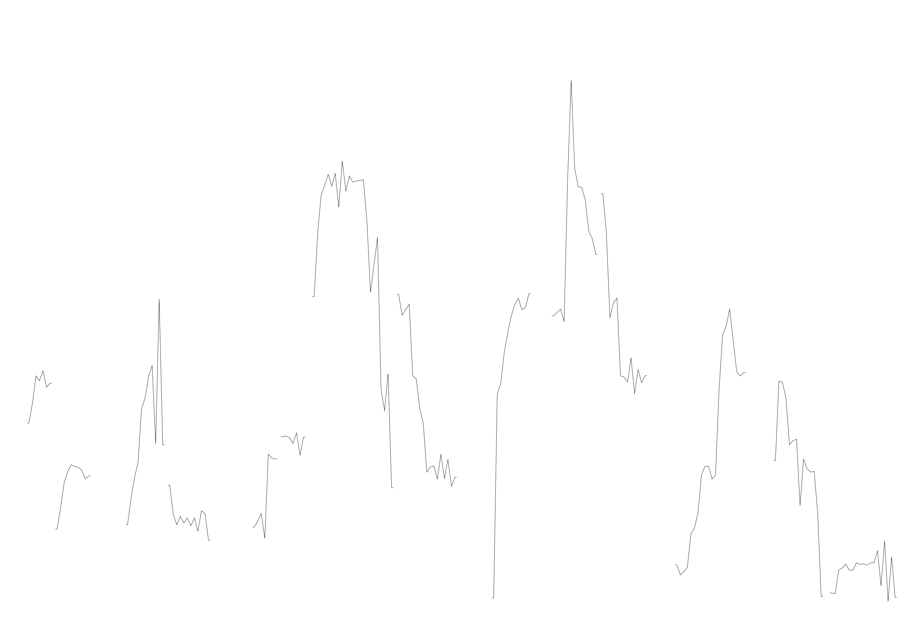
There is a whole lot of detail in the human performance that is not encoded in the Hertz data given above! What we realize is that even the concept of a “note” is itself a complex abstraction—trying to identify where a “note” begins and ends in a complex, raw frequency contour is quite difficult. We don’t really know exactly how humans do it!
The lesson here is that when analyzing musical encodings, we always have to consider:
- What knowledge is embedded in the data?
- What knowledge is missing from the data?
- What knowledge is needed to interpret the data?
Only by answering these questions can we reason intelligently about the validity of our analyses. Generally, as with other domains, raw qualitative measures are more complex and messy, but come with few preconceptions. On the other hand, quantitative data can be much easier to make sense of and analyze. After all, humans do perceive and conceptualize music in terms of “notes,” octaves, and tonal centers.
Symbolic vs Audio Data
Different fields and subfields of computational music research tend to focus on different types of data:
The field of computational musicology tends to focus on more quantitative data. This data consists of scores or “score-like” data, which we call symbolic data. This data tends to be infused with lots of domain knowledge.
In the Hey Jude example above, the
DegreeandScientificrepresentations are the most symbolic.The field of music information retrieval (MIR) tends to focus on more qualitative data. In particular, they study “raw” audio data, or data-driven features which are derived from the audio.
In the Hey Jude example above, the
Hertzand \(F_0\) representations are the most qualitative, as they contain lots of rich details and make few assumptions about the data. However, MIR researchers would probably want to directly study the full audio recording of Hey Jude, in all its complexity.
Note: in my experience, MIR researchers tend to view computational musicology as an interesting (but simplistic and niche) subfield of MIR. Similarly, computational musicologists tend to view MIR as a powerful (but grotesquely naive) subfield of computational musicology. They are probably both right.
Pieces or Performances
Traditionally, symbolic encodings of music have focused on representing musical pieces—like scores in the Western classical tradition—which exist independently of, and before, performance. However, encodings can also be used to represent performance-specific information as well. If we encode musical representations of an existing performance (after the fact), we call this a transcription. Most musicking traditions around the world are entirely oral, never “writing down” music in any sense. Even in Western music, most folk and popular music is not originally written down, though scores (e.g., guitar “tabs”) might be published after the fact. This makes transcription an essential research tool for most music research.
A transcription is an operational measurement of a performance, and may also be considered a measure of the abstract piece being performed. Thus, transcription has the same validity concerns as any other form of measurement. Transcriptions can contain systematic or random errors. Transcriptions can also be unreliable—compare five tabs of the guitar solo from Hot For Teacher (Van Halen) and you’ll observe many differences! Of course, score data can contain error too: for example, different editions of scores often have slight differences, including random mistakes made by editors.
Both scores and transcriptions (like guitar tabs) are used practically in Western performance and pedagogy. However, these emic scores and transcriptions are not created for research purposes. Rather, they mainly serve as performance aids, and they often contain systematic biases and assumptions that reflect this intended purpose. Most scores focus on representing the abstract, underlying piece, not exactly what is performed. Much information is missing from the score, like the details of timing, articulation, and dynamics; Performers must use their domain knowledge to fill in this information (“interpret” the score).
Performance scores are also usually optimized for ease of reading, rather than faithful representation of musical information. For example, Western notation rarely represents the duration of notes accurately; rather, a combination of pitch and rest note values is used to represent the onset times of notes as clearly as possible. Consider this bit of notation:
The top staff here is easy to read, and arguably represents the “true” abstract melody. The lower staff is a closer representation of what a musician might actually play.
Other notation traditions can be even more abstract and imprecise: like jazz lead sheets, Gamelan cipher notation, or guitar tablature. For example, if the same melody was treated as the “head” in a jazz lead-sheet, it might be performed like this:
Common Encodings
The most common music encoding scheme in the world, by far, is Western staff notation. Through the influence of Western institutions (e.g., Christian churches, European militaries) and technologies (e.g., piano, synthesizers, DAWs), Western models of pitch, rhythm, and “notes” have become common currency around the world. Most common digital notation schemes are essentially representations of Western staff notation—for example, musicXML and **kern.
The second most important coding scheme in the musical world is probably the Musical Instrument Digital Interface (MIDI) representation. MIDI, unlike staff notation, focuses on faithfully representing exact musical performances, including tiny details of timing and loudness.
Any transcription or encoding scheme makes implicit and explicit assumptions about musical structure—particular models of musical objects. It is important to be aware of what our encodings assume, in particular, what information they include and what they ignore. One fundamental assumption that is common to most music encodings is a focus on pitch and rhythm information—sometimes completely ignoring other musical information, like timbre.
Pitch
The organization of pitch is essential in most forms of music. There are a number of different ways to represent pitch in music research:
- F0
- Tonal pitch names (a.k.a., scientific pitch)
- Atonal (chromatic) pitch numbers (e.g., MIDI numbers, semitones)
- Scale steps
- Circle of fifths
- Scale degrees
- Pitch chroma
- Intervals
Each approach defines a “pitch space,” with a different numbers of levels, and different mathematical (and musical) properties.
Continuous pitch
The idea of “pitch” is closely related to the frequency-content of sound. However, the relationship between frequency content and percieved pitch is not trivial. Most sounds are perceived as “unpitched,” meaning that the perceptual quality of pitchedness is absent, or weak. In contrast, sounds with regular harmonic spectra are perceived as “pitched,” with a perceived “main pitch” being associated with the lowest frequency partial, called F0 (F zero, F naught).
Algorithms to extract continuous F0 contours from monophonic sound signals are fairly reliable and (perceptually) accurate (see the Hey Jude contour above). Calculated F0 is thus a common operational definition of the “pitch” in an audio signal. However, the “pitch” of a sound doesn’t always match the F0. For example, instruments like bells can have weird harmonic spectra, yet still sound pitched. Even human experts can disagree which frequency octave/harmonic is the pitch of a sound—in some cases, humans perceive “phantom” partials which don’t actually appear in the sound signal.
Discrete pitch
Human perception and cognition is often dominated by categorical processing. This is why, rather than a continuous, sliding F0 contour, we tend to perceive music as a sequence of discrete note events, each with its own (mostly) stable pitch. These stable pitches are also perceived categorically, ignoring (to some extent) vibrato and glissando between pitches. Symbolic music data rarely represent vibrato or glissandi, which may be excusable in Western classical music but is a known problem in genres like Hindustani and Carnatic music, where gamaka are essential to the music.
Most musical traditions draw pitch categories from a gamut of musical scales, described by a “tuning system.” In many cases, the relationship between a continuous F0 contour and the intended musical scales can be fairly obvious. However, this is not always the case, and even the best algorithms will fail or disagree with human interpretation at times. Do you think you could reliably turn the Hey Jude F0 contour above into one of the symbolic representations, algorithmically? Perhaps not. However, if you ask human experts to listen to Hey Jude and write down the discrete note categories, you’ll find little (if any) disagreement. This is why expert human transcription (or validation of output) is still valuable. Of course, there is plenty of music where human experts will have disagreements about pitch categories: Try transcribing something like Get Up by James Brown—I transcribed this for CoCoPops, and it was not easy! Musical practices like glissandi, gamaka, and “blue notes” (Temperley, Ren, and Duan 2017) still represent significant theoretical and practice challenges to music research.
There are two prominent, widely-used pitch-category gamuts: tonal “note names” and atonal (chromatic) semitones. Semitones are a modern invention, dividing frequency space into logarithmically equal steps—twelve per octave. They are often represented simply as integers, with most of the associated mathematical properties of integers on an interval scale. MIDI note numbers are semitones, with the note-value 60 pegged to C4 (middle C); music theorists often center semitones with 0 as middle-C.
Note: Any discrete pitch representation can be amended with “cents” information (representing one hundredth of a semitone), or MIDI “pitch bend” information, to achieve something closer to a continuous pitch data.
Semitones are a relatively “raw” measure, as they ignore important perceptual and structural features of music, like octave and tonality. They are indeed, atonal. In contrast, traditional Western note names—like similar systems in other cultures—encode much more musical information. The Western pitch system is based on the seven-note diatonic scale, labeled (because of weird accidents of history) C-D-E-F-G-A-B, with the addition of possible “accidentals” to alter the scale. These scale steps do not correspond to equal steps in log-frequency or semitones; instead, there are five larger steps (whole steps) and two smaller steps (minor steps). However, humans do perceive them as equivalent “steps”: non-musicians will generally find it difficult to identify which steps are smaller and which are bigger. Steps can be represented reasonably as integers—however, full tonal names (e.g., with accidentals) cannot be because they are usually considered a partially ordered set: e.g., E4 is above D4 but Eb is neither above nor below D#.
The importance of tonality and the tonal center leads to the creation of alternative representations of tonal pitches, wherein scale-steps (and/or accidentals) are indicated relative to the tonic note. Scale degrees can be indicated by natural numbers 1–7, with or without accidentals; Roman numerals I–vii are often used to represent scale-degree “roots” of harmonies. Be careful doing math with scale degrees: there is no zeroth scale degree. Systems of solmization—like Western solfege, Japanese Iroha, and Hindustani svara—are essentially similar to Western scale degrees (though the scales themselves may be different).
Chroma
Human perception and our musical traditions tend to regard frequencies related by ratios corresponding to powers of 2 as “the same” (to some degree). This is called octave equivalence.
For many musical analyses, octave or “pitch height” is irrelevant, and we want to work with pitch representations that are octave-invariant: pitch chroma. For example, \(424_{Hz}\) and \(848_{Hz}\) correspond to different pitches, but are the same pitch chroma. In contrast, \(424_{Hz}\) and \(954_{Hz}\) are different pitch chroma.
When talking about categorical pitch, music theorists refer to octave-invariant categories as pitch-classes. This terminology is usually used in the context of atonal semitones. Basically, all semitone values (or MIDI numbers) are treated modulo 12, so there are only values 0–11. (C = 0, G#/Ab = 8, B = 11, etc.) Music theorists often encode pitch-classes 10 and 11 as t and e respectively, to avoid confusion with 1 and 0.
Tonal pitch chroma can be represented without ambiguity as integers on the line-of-fifths, or “wrapped” into 12-tone equivalence on the circle-of-fifths. This is an excellent representation for tonal information when pitch contour and pitch height are irrelevant. Intervals on the line-of-fifths are equivalent to unique tonal intervals, for example,
- \(+4\) is a major third.
- \(-4\) is a minor 6th (inversion of major third).
- \(+7\) is “sharpen.”
- \(-7\) is “flatten.”
- etc.
To summarize, our octave-invariant symbolic representations:
| … | F- | C- | G- | D- | A- | E- | B- | F | C | G | D | A | E | B | F# | C# | G# | … | |
|---|---|---|---|---|---|---|---|---|---|---|---|---|---|---|---|---|---|---|---|
| Line of fifths | … | -8 | -7 | -6 | -5 | -4 | -3 | -2 | -1 | 0 | 1 | 2 | 3 | 4 | 5 | 6 | 7 | 8 | … |
| Circle of fifths | … | 4 | 5 | 6 | 7 | 1 | -3 | -2 | -1 | 0 | 1 | 2 | 3 | 4 | 5 | 6 | 7 | 1 | … |
| Pitch class | … | 4 | 11 | 6 | 1 | 8 | 3 | 10 | 5 | 0 | 7 | 2 | 9 | 4 | 11 | 6 | 1 | 8 | … |
Remember that this form of data ignores pitch height, which means that the “contour” of melodies cannot be faithfully extracted. If you observe a sequence like “G A D E C” you don’t know whether the transition “A -> D” went up or down in scale space.
Distance Metric
Notice that different representations of pitch necessarily imply different distance metrics. In all of our integer based representations (MIDI, semitones, line of fifths), we can simply calculate the difference between the values to get a distance, but we get different distances in different representations. However, for “circular” representations of pitch classes, we typically take the shortest distance on the circle. For non-integer representations, distance metrics may be categorical, or partially ordered. For example,
- The distance between C4 and G4 is…
- \(1\) on line of fifths.
- \(7\) in semitones.
- \(5\) in pitch class space (\(12 - 7\)).
- “Perfect fifth” in tonal names.
- The distance between C4 and G#4 is…
- \(8\) on line of fifths.
- \(8\) in semitones.
- \(4\) in pitch class space (\(12 - 8\)).
- “Augmented fifth” in tonal names.
- The distance between C4 and Ab4 is…
- \(-4\) on line of fifths.
- \(8\) in semitones.
- \(4\) in pitch class space (\(12 - 8\)).
- “Minor sixth” in tonal names.
- The distance between C4 and Ab3 is…
- \(-4\) on line of fifths.
- \(-4\) in semitones.
- \(4\) in pitch class space (\(12 - 8\)).
- “Descending major third” in tonal names.
- The distance between C4 and B3 is…
- \(5\) on line of fifths.
- \(-1\) in semitones.
- \(1\) in pitch class space (\(12 - 11\)).
- “Descending minor second” in tonal names.
Relative pitch
Most human beings cannot recognize or remember specific frequencies/pitches. Human musical systems reflect this reality, focusing on relative pitch relationships. For example, in Hindustani music, musicians more or less pick any comfortable pitch they want to function as sa (tonic), tune their instruments to that pitch, and play. Most musical systems operate the same way.
Note: The Western system of pitch representation also began relative: In medieval or Renaissance music, we have little idea what frequency middle-C would have corresponded to, as it would have been up to the local musicians. Thus, Western scores from earlier eras don’t actually represent absolute pitch at all. The Western pitch gamut stabilized on twelve-tone equal temperament only in the mid-19th century, with the tonal pitch gamut tuned exactly like the atonal 12-semitone gamut, and with A4 pegged by convention to \(440_{Hz}\). It is mistake to assume, that middle-C (C4) is just another way of saying \(261.6256_{Hz}\).
One way to “relativize” pitch data is by relating each pitch to a reference pitch, like the tonal center. This is what scale-degree representations do. Another approach is to look at the melodic intervals between successive pitches. For example, Hey Jude could be encoded like this:
   Atonal.Intervals Tonal.Intervals Lyrics
1               [c]             [c]    Hey
2                -3             -m3  Jude,
3                 0              P1  don't
4                 3             +m3   make
5                 2             +M2     it
6                -7             -P5   bad.
7                 0              P1   Take
8                 2             +M2      a
9                 1             +m2    sad
10                7             +P5   song
11                0              P1    and
12               -1             -m2   make
13               -4             -M3     it
14                2             +M2   bet-
15               -2             -M2  -ter.
16               -2             -M2      _
17               -1             -m2      _
18                0              P1    Re-
19                1             +m2  -mem-
20                0              P1   -ber
21                0              P1     to
22                9             +M6    let
23               -2             -M2    her
24               -1             -m2    in-
25                1             +m2    -to
26               -3             -m3   your
27               -2             -M2 heart.
28               -7             -P5   Then
29                2             +M2    you
30                2             +M2    can
31                5             +P4  start
32               -2             -M2      _
33                0              P1     to
34               -2             -M2   make
35               -1             -m2     it
36               -5             -P4   bet-
37                1             +m2   -ter
This is an unfamiliar way of encoding pitches, at least for most Western musicians. However, given that (most) humans only perceive pitch relatively, this might be a closer representation of how humans perceive pitch in music.
Case study
Let’s say we want to measure and encode musical from an unfamiliar culture. How should we go about doing this? What many early, imperialist, ethnomusicologists did was write down the pitches using modern, absolute Western notation. They might, for example, take an unfamiliar instrument measure the frequencies (F0) it produces and write them down as:

What do we think of this attempt to measure the culture’s scale? It might be fine as a very raw representation, as it would allow us to reproduce the exact fundamental pitches of the instrument; If you’d like to program a Western synthesizer to play the scale, it would be perfect. However, it tells us nothing about the organization of the scale or the music. What’s worse, it includes a lot of useless information and Western bias. It is very unlikely that the musicians who play this scale think of the bottom note as a “flattened” version of another note. In fact, its likely that the absolute pitch height is totally irrelevant: for all we know, the exact tuning of the instrument might change with each performance.
This transcription makes another, more subtle assumption as well. The ethnomusicologist assumes that a seven-note scale is the norm, and writes this five-note (pentatonic) scale down with gaps where the other two steps are “supposed” to be. However, many cultures around the world use pentatonic scales and they don’t consider themselves to be “skipping” any notes. Indeed a pentatonic scale can be constructed from five perfect fifths, resulting in a scale with two large and three small steps. The large steps will correspond to skips (3rds) in a diatonic scale, while the smaller steps correspond to diatonic whole steps. However, from the emic (within-culture) perspective, they are simply large and small steps, just like the large and small steps of a diatonic scale. Assuming that there are “supposed to be” two additional notes there, is baseless.
Rhythm
The organization of time is essential in most forms of music. There are a number of different ways to represent timing in music research:
- Milliseconds
- Durations
- Inter-onset-intervals
- Beats
- Metric position
Each approach defines a “rhythmic space,” with a different numbers of levels, and different mathematical (and musical) properties.
Onsets and Offsets
As mentioned above, most rhythmic representations focus on the onsets of musical events: when they begin. Offsets—when events end—are often ignored or recorded with less detail. Not all musical events have well defined onsets (or offsets), and representing their timing precisely can be rather arbitrary. The percieved onset of an event can often differ significantly (on the order of \(50--200_{ms}\)) from the acoustic onset.
Staff notation focuses on the duration of events: the time between onset and offset. This requires the addition of additional “rest” objects, to indicate the duration of silences between note events. Another approach is to look at the interval between successive onsets: inter-onset-intervals (IOIs). Most musicians conceptualize rhythmic patterns (at least implicitly) in terms of IOIs. However, using IOI representations of rhythm necessarily ignores duration information, and thus the presence (if any) of rests/silence. This may or may not be appropriate, depending on your research goals.
Note that, when you calculate IOI data, the IOI of the last rhythmic event is ill defined.
All musical “note” events unfold over a span of time. However, humans tend to perceive notes (and syllables) as having a single rhythmic “center,” called the perceptual center (or “P-center”) in linguistics research. The perceptual center is roughly correlated with the amplitude peak in most sounds, but this is not always the case.
Onsets, P-centers, and offsets are all a bit fuzzy and complicated, so measuring them always involves measurement error. Automated approaches to detecting onsets are fairly accurate (at least, for monophonic signals), but can differ from human perception in many cases. Asking human annotators or scribes to annotate onsets/P-centers/offsets can result in more accurate data, but obviously is much slower (and has other issues). Human expert scribes can create conventional rhythmic transcriptions; however, another approach is to annotate audio recordings directly using software like Praat, Sonic Visualizer, or even a commercial DAW. It can be very effective to playback your own onset annotations (e.g., as click sounds) along with the original audio, so you can hear how well they match.
As always, the take away message is to never regard any rhythmic data as objective—always be skeptical of the construct validity of rhythmic data.
Continuous time
The timing of events (usually their onsets or P-centers) can be represented precisely using standard units of time. Seconds, milliseconds, etc. It is generally preferable to measure everything in seconds or milliseconds. Using combined representations like 2:34 is nice because they are easier for humans to interpret, but they can be ambiguous (is that hh:mm, or mm:ss) and are harder to program with.
Absolute time markers are rarely used with score data, but common for measurements of performances (audio recordings). Time is usually measured from the beginning of an audio recording, as an absolute reference. These are called timestamps. This approach is very “raw,” potentially including a lot of detail.
Watch out for (inconsistent) amounts of silence at the beginnings of recordings! Often different releases of “the same” song will have different amounts of silence, which can throw off time stamps. We can also measure the time between onsets, or between P-centers.
MIDI data encodes time on a scale of discrete “ticks,” usually a specific number of pulses per quarter note (PPQ). MIDI performance data often uses PPQ or 480 or 960, achieving essentially continuous time resolution.
Discrete time
Musical time is generally conceptualized and perceived categorically. The durations of rhythmic events are associated with a small number of categories, with the relative duration of categories related by simple ratios. These categories are represented as rational “note-values” in staff music: whole, half, quarter, eighth, etc.
Rhythmic durations in most music are related to a constant, isochronous pulse: the “main beat” or tempo. In order to determine the absolute timing of events from a score, you need to know the tempo. This is problematic because 1) traditional scores include no exact tempo indication, 2) tempo can vary, and 3) datasets sometimes omit the tempo information.
As mentioned above, extracting “clean,” score-like rhythmic notation from continuous timing data is quite difficult. Most measurement procedures—whether computational or based on human annotation—probably have error at least in the \(\pm 10_{ms}\) range. Note that small changes in timing, in the 1–\(15_{ms}\) range, are difficult for humans to perceive accurately at all.
The timing of actual human performance also varies, both systematically and randomly, from categorical ideals. If you take a MIDI recording of a human performance and drop it into a score editor, you’ll often see something like this:
In this case, it would be fairly easy to algorithmically “quantize” this MIDI data to match the “correct” onset times of the intended melody. However, getting the correct, clean offsets is much harder. What’s worse, most MIDI performance data—or any equivalent continuous timing data—is much messier than this, and getting the right onsets is also difficult. How do you differentiate a “rushed” downbeat from a syncopation? It’s harder than you would think! This is where human expert transcription comes in handy—though human experts will definitely disagree about rhythmically complex music.
Meter
The rhythmic organization of many musical cultures is centered around a repeating pattern of interlocking beats. The position of rhythmic onsets within the meter can be the most significant aspect of how rhythms are perceived. For example, “the same” sequence of rhythmic durations can be perceived quite differently when set to a meter in different ways (Acevedo, Temperley, and Pfordresher 2014). Unfortunately, good systems for encoding rhythms in a meter-informed way have not been devised. We usually must infer/interpret metric position and strength from a sequence of rhythmic durations or IOIs.
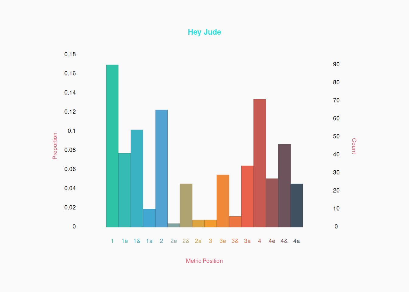
Many projects restrict their analyses to simple duple meter (e.g., 4/4 time), simply because considering other meters adds a lot of complexity. Duple meter is often analyzed as 16 or 32 metric positions.
Getting Encodings
Musical encodings don’t grow on trees. We need to find them, or make them!
Over the last fifty years, a number of large repositories of symbolic music data have been assembled. Notably, the website Kern Scores includes many of these repositories. Generally, these repositories are heavily biased towards European music, especially European classical music. They also tend to be heavily biased towards note information, often omitting other score details, like dynamics and lyrics. These sorts of existing repositories represent convenience samples, which have historically shaped (and constrained) the field of computational musicology.
Most symbolic music datasets have been created by copying existing scores (on paper or in digital images) into a machine-readable format, like humdrum. This usually meant endless hours of tedious work by human volunteers. More recently, advances in optical music recognition (OMR) have made going from a score-image to a machine-readable notation much faster. However, to achieve high-accuracy, it is still often necessary for a human expert to correct the output of OMR systems.
Obtaining encodings or annotations of musical performances (i.e., transcriptions) is even more difficult and time consuming than encoding scores. Most existing datasets have been transcribed by human experts; for example CoCoPops. Automated approaches to extracting pitch and rhythm information have advanced rapidly in the last decade. However, creating “clean,” score-like transcriptions is still a major challenge. In other words, automatically extracting performance information (like F0) is easier than automatically extracting piece information.
Human annotators and scribes are usually (necessarily) music “experts” in some sense, who must be recruited and vetted. Some tasks may only be trusted to particularly skilled musicians, or academics with significant training (i.e., graduate degrees in music theory). However, non-experts (even lay people) may be useful annotators for other tasks, like genre or emotion labelling.
If you are recruiting human annotators or scribes—either as volunteers or paid labor—, you may need IRB approval.
Annotations
Annotations about music—like chord or genre labels—are generally easier to get than actual note-information, simply because there are usually far fewer objects to annotate. For example, most music has far more “notes” in it than “chords,” so labelling all the chords in a song takes a lot less time than transcribing all the notes. Many audio features can be reliably and quickly computed algorithmically. However, good annotation of more musical information still relies on human annotators more often than not. Human annotations have served as the “ground truth” used to train many machine learning models.
Construct Validity
Whether using humans or algorithms, we must always consider the construct validity of our transcriptions/annotations. How accurate are our annotations? How reliable?
For automated systems, reliability is usually high—deterministic algorithms will give the same output every time. However, accuracy can be low. When using automatic transcription or annotation systems, you should always manually inspect the output of a large, random sample of cases. How often does the system make random errors? Does the system make non-random errors, like mislabeling minor chords more often than major chords? Etc. Don’t cherry pick successful examples—try to get a realistic picture of how well (or how poorly) the annotation/transcription algorithm performs. Only then can you hope to make valid claims based on your data.
For human annotators, the greatest concern is reliability. If you ask five music theorists to do harmonic analyses of a piece of music, you’ll get five slightly different analyses. Some of this disagreement is due to random errors. However, often the problem has to do with definitions: each annotator has a (subtly) different idea of what “harmonic analysis” means. For example, some theorists will explicitly label a lot of chordal extensions (e.g., C9, G9#11) while others will leave them off because they are non-harmonic tones. This is why the most important thing when working with human annotators is giving precise instructions, including precise definitions of all terms. Tell your annotators exactly how they should interpret things, or be willing to accept greater variance in their responses.
One standard practice is to have multiple independent annotators for all data. This allows you to identify disagreements and inconsistencies, and thus assess inter-rater reliability. For example, David Temperley and Trevor de Clercq (2011) each independently transcribed the harmonies of the 200 songs in their Rolling Stone dataset; Similarly, when we were grad students, Claire Arthur, Kirsten Nisula, and I worked together to create two separate harmonic transcriptions for each piece in the TAVERN dataset (Devaney et al. 2015). When you have multiple independent annotations (or transcriptions), you can either consolidate them—for example, averaging them together (if that makes sense) or reviewing and correcting disagreements—or simply publish all the independent annotations.
In real research, validity concerns must be balanced with practicality. Algorithmic transcriptions may make more mistakes than a human expert, but can be run tens of thousands of times faster. You can also save a lot of time by only measuring limited annotations. Do you really need to transcribe every note in the song? Or do you just need to find and annotate the lowest and highest notes? This would be much easier for a human to do, and much quicker.