Probability can be transformed into other, equivalent forms. In some cases, these other forms can be more intuitive, or mathematically tractable.
Log probability/likelihood
I have gathered two samples of data: each sample consists of 100 independent observations. I want to know which of the two samples better fits a standard normal distribution. To do this, I can compute the likelihood that each sample came from a standard normal distribution:
  [1] 5.475847e-02 4.526115e-02 7.627397e-03 4.013628e-02 3.308118e-02
  [6] 8.949329e-03 4.689743e-02 2.736809e-02 1.095884e-02 1.071145e-02
 [11] 2.520956e-02 4.344873e-04 4.397269e-02 1.987591e-03 4.729322e-02
 [16] 9.241579e-03 3.683368e-02 3.206991e-02 7.092941e-03 4.334564e-03
 [21] 7.573589e-02 5.195933e-03 8.846074e-03 7.330947e-02 1.026664e-04
 [26] 8.046441e-37 1.785157e-04 3.899997e-02 2.366669e-02 2.461940e-02
 [31] 1.302043e-02 1.368127e-04 2.149305e-02 2.245061e-02 7.271579e-03
 [36] 4.104999e-02 2.044704e-02 3.741629e-02 1.395583e-02 2.615802e-02
 [41] 3.909264e-03 1.775987e-01 9.827064e-03 1.177354e-01 1.742598e-02
 [46] 5.737425e-02 3.683230e-02 1.129464e-01 1.090845e-04 3.520984e-08
 [51] 3.578341e-02 3.913806e-02 1.932899e-01 2.962960e-02 2.999773e-02
 [56] 2.706426e-02 4.055382e-02 6.122257e-02 4.459003e-02 1.413320e-02
 [61] 6.216708e-05 1.344381e-02 2.035670e-03 6.092102e-02 1.212940e-78
 [66] 1.280266e-02 9.676168e-03 3.745478e-02 3.004656e-02 6.163392e-09
 [71] 1.285420e-02 1.920484e-02 8.676673e-03 3.024075e-02 7.569453e-02
 [76] 9.116563e-02 1.558412e-06 8.582833e-02 2.607782e-02 4.011581e-02
 [81] 7.475858e-03 3.166966e-02 6.734173e-03 1.098028e-02 1.097438e-01
 [86] 1.300855e-02 1.988106e-01 7.231250e-02 4.864303e-02 3.067038e-02
 [91] 1.404320e-01 1.205429e-01 2.340505e-02 6.611165e-02 4.824871e-04
 [96] 4.202558e-03 4.984495e-02 2.671472e-02 3.087060e-02 2.318005e-02
  [1] 4.861293e-02 6.453214e-02 1.002729e-02 3.008977e-03 1.611607e-01
  [6] 1.343832e-02 2.087271e-02 8.294782e-02 5.196236e-03 7.903034e-02
 [11] 6.814081e-02 6.661713e-03 4.850578e-04 2.592891e-02 8.260927e-02
 [16] 1.704382e-01 7.288886e-02 1.436646e-01 6.562971e-02 2.001513e-02
 [21] 1.332649e-01 1.251703e-05 3.243472e-02 3.151481e-03 1.724905e-01
 [26] 8.963190e-03 1.815621e-01 5.650498e-03 1.985464e-02 8.100856e-02
 [31] 1.768508e-03 1.150897e-01 1.006791e-01 1.506898e-01 1.111078e-01
 [36] 5.278588e-03 1.838237e-02 4.482668e-03 7.912516e-02 2.079982e-02
 [41] 2.731191e-02 1.892871e-01 3.948548e-04 3.378774e-02 8.427923e-03
 [46] 5.138634e-03 4.706978e-02 7.030444e-02 6.056695e-03 1.558314e-01
 [51] 1.962224e-04 7.842862e-02 6.074818e-04 9.749723e-04 3.718063e-02
 [56] 1.361147e-02 1.533204e-01 2.326597e-02 4.029065e-03 3.609390e-02
 [61] 8.614561e-02 1.096192e-01 4.590796e-02 3.750293e-03 8.950190e-02
 [66] 5.292446e-02 1.797857e-01 1.607394e-02 1.859465e-03 1.024323e-03
 [71] 7.439618e-03 1.980451e-01 1.652198e-02 1.749915e-02 7.522053e-02
 [76] 3.154861e-02 1.347207e-01 1.043420e-02 7.248276e-02 1.962332e-01
 [81] 7.670358e-02 1.561766e-03 7.322522e-02 9.149010e-03 5.258693e-03
 [86] 4.280745e-02 7.510733e-02 9.473638e-02 8.994761e-03 1.575904e-01
 [91] 2.720065e-02 6.865806e-02 1.747077e-01 1.881949e-01 5.707836e-03
 [96] 5.919659e-02 7.660230e-03 2.671512e-04 1.104027e-03 1.048403e-02
However, to calculate the overall likelihood of each sample, I need to know the joint probability of the 100 observations in each sample. Since we know that the observations are independent, the joint probability is simply their product, which is (according to R):
- Joint likelihood of sample 1: 0.
- Joint likelihood of sample 2: 0.
Wait…that can’t be right can it? There shouldn’t be any zeros. What has happened is that the numbers are too small for my computer to represent.
If we shrink our sample size a little, by using only the first 50 numbers from each sample, we can get numbers:
- Joint likelihood of first 10 observations from sample 1: 1.3544749^{-42}.
- Joint likelihood of first 10 observations from sample 2: 4.659095^{-40}.
Still tiny numbers, but at least we can compute them. We can now answer our question by looking at the ratio between the two numbers—the likelihood ratio:
\[
\frac{P(sample_1)}{P(sample_2)} = LikelihoodRatio
\]
In this case, the likelihood ratio is 0.0029. The first sample is much less likely (3 out of 1000 chance) to have come from a standard normal distribution, compared to the second sample.
But, it is problematic that we had to throw away most of our data! This estimate would be much more accurate if we could use all the data.
When working with actual data, we almost always encounter likelihoods that are too small to compute. To get around it, we often work with the logarithm of likelihoods: the log-likelihood. We’ll always use the natural log, using a base of \(e\), so it’s \(\log_e(p)\).
When we transform our likelihoods to a log scale, the operation of multiplying probabilities is transformed to the operation of adding log-probabilities. Thus, instead of multiplying all the independent likelihoods together to get the joint likelihood, we can add all the log likelihoods together to get the joint log likelihood. The joint log-likelihoods for the two samples (using all the data points) are:
- Joint log-likelihood of sample 1: -2220.494808.
- Joint log-likelihood of sample 2: -980.8606848.
Now, just as multiplication is converted to addition on the log scale, division (or ratios) are converted to subtraction. So we can calculate the log-likelihood ratio by subracting these two numbers:
\[
\log(P(sample_1)) - \log(P(sample_2)) = LogLikelihoodRatio
\]
In this case, the log-likelihood ratio is -1239.6341.
Note: most of the time when we talk about likelihoods and “likelihood ratios” in research, we are actually referring to the log-likelihood and log-likelihood ratio.
Other note: the entire analysis here hinges on the fact that the joint probability of independent observations is simply the product of their separate probabilities. As we now know, this is the same as the sum of the log of their probabilities. However, if the data points are not independent then the whole idea breaks down!
Odds
“Odds” are an alternative formulation of probability. Remember, odds convey the exact same information as probability, just in a different form.
- \(odds = \frac{p}{1 - p}\)
- \(\frac{odds}{odds + 1} = p\)
Odds can be any positive real numbers, bounded in the range 0 to \(\infty\) inclusive.
\[
0 \leq odds \leq \infty
\]
- If \(p = 0\), the odds are \(0\)
- If \(p = 1\), the odds are undefined!
- They might show up as \(\infty\) in some software.
Odds are often expressed as ratios: like “4-to-1” or “1-to-4.”
\[
odds(p = .2) = \frac{1}{4}
\]
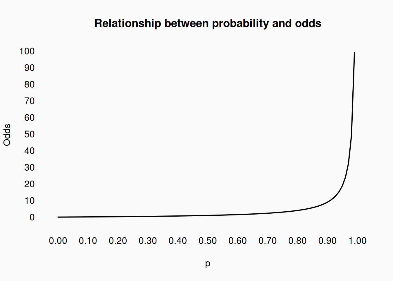
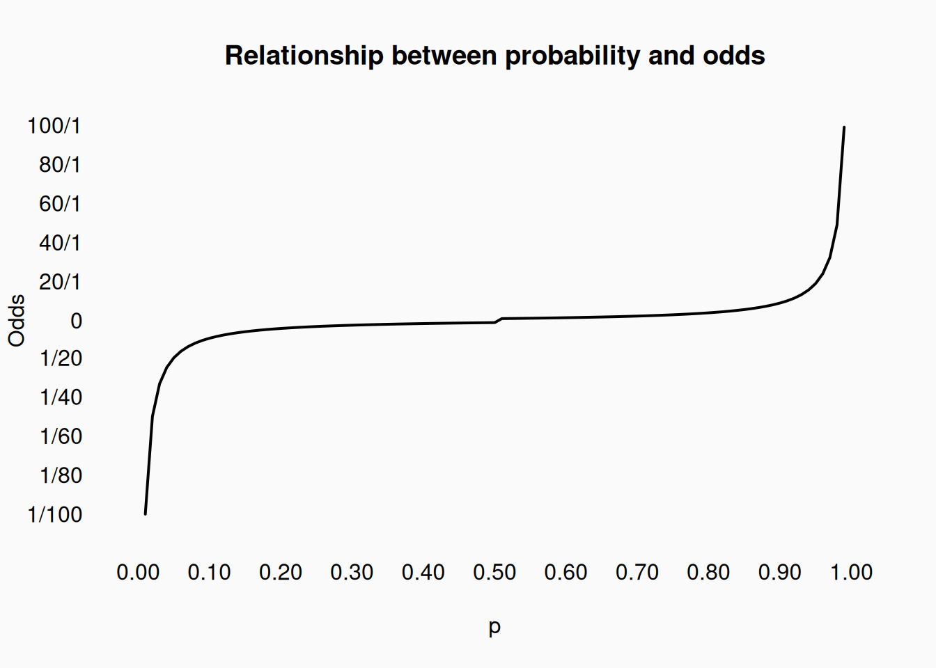
This graph shows how odds approach \(\infty\) as \(p\) approaches \(1\). However, it doesn’t show that odds are reciprocally symmetrical around \(p = .5\). This means that
\[
odds(1 - p) = \frac{1}{odds(p)}
\]
This symmetric makes the most sense if we express odds in ratios. For example:
\[
odds(p = .2) = \frac{1}{4}\\
odds(p = .8) = \frac{4}{1}
\]
\[
odds(p = .25) = \frac{1}{3}\\
odds(p = .75) = \frac{3}{1}
\]
\[
odds(p = .08) = \frac{2}{23}\\
odds(p = .92) = \frac{23}{2}
\]
We can graph this by tweaking our Y-axis: