| Coefficient | |
|---|---|
| \(b_0\) | 1.793 |
| \(b_1\) | 1.693 |
48 Linear Models
(Modified on 2026-08-12)
458 words
The vast majority of statistical models used in research are linear models.
What does “linear” mean in this context? Intuitively, it means that the relationship between variables makes a straight line in a graph. A more formal way to put it is that the relationship is unchanged by scaling. If we notate the “the relationship between \(X\) and \(Y\)” as \(X \sim Y\) and then pick any arbitrary number as \(a\), then:
\[ a (X \sim Y) = aX \sim aY \]
In other words, the relationship between \(X\) and \(Y\) isn’t really affected by the multiplication by \(a\). If you try this with non-linear relationships1, you’ll see that this doesn’t work.
Obviously, relationships in the real world are rarely going to be strictly linear, and using linear models may thus represent a failure of construct validity. However, linear models are surprisingly flexible—and can be quite complex and sophisticated—and have proven themselves time and again to by “good enough” models for many research purposes (All models are wrong, but some are less wrong). Above all else, linear models are used because they are well understood, easy to compute, and easy to interpret—these are major advantages.
Linear models can be used in both descriptive and inferential ways.
- The basic statistics we commonly use to describe relationships between samples of numbers—things like “covariance” and “correlation”—are all linear.
- We can also postulate that the “true” relationships between variables in the real-world statistical populations we are studying feature linear relationships. In this case, we claim that the statistics in our linear models are inferential estimates of population parameters.
Simple Linear Relationships
“Simple” linear models involve only two variables, which we will call \(X\) and \(Y\). As a starting point, we will assume that \(X\) and \(Y\) are both numbers on a continuous, ratio scale. We’ll consider other possibilities below.
Covariance
As we know, a basic property of random variables is that they…vary. That is, their value is different each time they are observed (sampled). This variation can be described in many ways; One of the most basic descriptors is the variance, which is a measure of how “spread” a variable is around its central tendency (mean).
When we consider two random variables, we can ask: how much do they vary together? Is their variation independent or dependent, or some of both? One way to characterize any linear dependence between variables is with the covariance—which is related to the variance. The variance (\(\sigma^2\)) of a variable is the average squared deviation from its mean (\(\mu\)):
\[ Var(X) = \sigma_X^2 = E((X - \mu_X)^2) \]
To understand the equation for covariance, below, let’s first rewrite this variance equation without the exponent:
\[ Var(X) = \sigma_X^2 = E((X - \mu_X) \times (X - \mu_X)) \]
This clarifies that we multiply \((X - \mu_X)\) with itself to get the variance. What if we instead multiplied it by another variable?:
\[ Cov(X, Y) = \sigma_{XY}^2 = E((X - \mu_X) \times (Y - \mu_Y)) \]
This is the covariance. As you can see, it is essentially the same idea as variance; In fact, variance is just a special case of “self covariance.”
Unlike variance, which is always positive, covariance can be positive or negative:
- When both variables are above their average (\(x > \mu_X\) and \(y > \mu_Y\)), both \((x - \mu_X)\) and \((y - \mu_Y)\) are positive and their product will be too.
- When both variables are below their average (\(x < \mu_x\) and \(y < \mu_Y\)), both \((x - \mu_X)\) and \((y - \mu_Y)\) are negative, so their product will also be positive.
- When the two variables are opposite sides of their average, one is positive and the other is negative, resulting in a negative product.
If two variables tend to agree, the covariance will be positive. If two variables tend to disagree, their covariance will be negative. If two variables agree and disagree equally, their covariance will be zero.
Covariance is one of the most basic ways we can describe linear relationships between variables, and it is a very important descriptive statistic. As a descriptive statistic, we’ll notate the covariance between \(X\) and \(Y\) as \(s_{XY}\).2
Unfortunately, the covariance isn’t very descriptive by itself, because it is difficult to interpret. Being based on the product of two variables, the scale of covariance can be hard to make sense of.
- Is a covariance of \(0.2\) big or small?
- Is a covariance of \(1,392,062\) big or small?
- It’s hard to say!
Usually, we compare covariances computed from similar variables, so that their comparison makes sense. Another approach is to normalize the covariance, by rescaling it to a more useful scale, as we’ll read more about below.
Linear regression
Let’s consider a more conceptual, approach to linear modeling, more suited to inference.
A basic linear model relates an independent variable \(X\) to a dependent variable \(Y\) like this:
\[ Y = \alpha + \beta X + \epsilon \]
\[ \epsilon \sim \mathbb{N}(0, \sigma) \]
- \(\alpha\) (alpha) is the intercept of the model.
- This would be the “baseline,” mean value, if there was no effect from \(X\), or where \(X = 0\).
- \(\beta\) is the regression coefficient, describing the relationship between \(X\) and \(Y\).
- Regression coefficients are also called regression “slopes.”
- \(\epsilon\) is a random variable representing residual error.
- We are assuming this error is normally distributed.
- \(\sigma\) is the standard deviation of the residual error.
Notice we are assuming that \(Y\) is a continuous numeric variable on an unbounded ratio scale. When both \(X\) and \(Y\) are continuous numeric variables, we call this a linear regression model.
The null hypothesis (\(H_0\)) for this model is that \(\beta = 0\). If \(\beta = 0\), then the effect of \(X\) disappears, so all that’s left is the intercept, which will be the mean value of the error distribution.
\[ \alpha + 0 * X + \epsilon= \alpha + \epsilon = \epsilon \sim \mathbb{N}(\alpha, \sigma) \]
Interpretation
A regression coefficient represents a value that transforms (as well as it can) \(X\) into \(Y\). This means that, unlike the covariance, a regression coefficient can be interpreted on the scale of \(X\) and \(Y\). The regression coefficient can be interpreted as:
For every one-unit change in \(X\), the average value of \(Y\) changes by \(\beta\).
It turns out that the regression coefficient is closely related to the covariance. In a simple regression, the regression coefficient is actually the covariance divided by the variance of \(X\):
\[ \frac{\sigma_{XY}}{\sigma^2_X} = \frac{Cov(X,Y)}{Var(X)} = \beta \]
To illustrate the interpretation of regression coefficients, let’s consider an example. We will investigate the linear relationship between “the size of melodic intervals between notes” and “the duration of notes,” using the first ten chorales by J.S. Bach as a convenient sample. A priori, I predict that longer durations are more likely to have larger melodic intervals. We can view this problem as a simple regression where \(Y\) is the absolute melodic interval (in semitones) and \(X\) is the duration in (whole notes). If we estimate the regression coefficients of this data we find:
Notice that we use \(b_0\) and \(b_1\) because these are statistics calculated from the data, and only estimates of the “true” parameters.
The covariance between melodic interval and duration is 0.019, but this is not interpretable. In contrast, we can directly interpret these \(b\) coefficients as follows:
The \(b_0\) estimate indicates that when the duration is zero, the average melodic interval size would be 1.79—this is the “baseline.”
- This intercept doesn’t make much sense, because rhythmic durations are never zero.
The \(b_1\) estimate indicates that for every one unit change in duration, the average interval size changes by 1.69. We are measuring duration in whole notes, so that means a change of one whole note predicts a change in average interval size of 1.69.
In these chorales the vast majority of notes are eighth-notes and quarter-notes, so a difference of one whole note is enormous on the scale of our data.
These examples illustrate that we need to be careful interpreting linear regression beyond the bounds of our variables. The mathematical model doesn’t “know” that durations are always positive, or that whole notes are rare, but we do.
Scale
A simple regression coefficient is just a rescaling of the covariance. More generally, if our numeric variables are on a ratio scale, we can consider other ways to rescale them to make the coefficients easier to interpret.
I mentioned above that whole notes are kinda big units for chorale music. What if we change our unit of duration to quarter notes and recalculate our coefficients? There are four quarter notes per whole note, so we just need to multiply \(X_{whole} * 4 = X_{quarter}\). If we do this the \(\beta\) will need to be divided proportionally (by four) to get the same \(Y\) prediction. \(\beta\) has to change reciprocally to the change in \(X\) unit.3 This means, that if we recomputed \(b\) using quarter notes, the estimate will be one quarter of the whole-note estimate: 0.42. Thus,
A quarter-note change in duration predicts a change in average melodic interval size of 0.42 semitones.
Notice that this hasn’t actually changed anything about the relationship between the variables, it has just changed the scale. You can use whatever scale of \(X\) is most intuitive.
What if we rescale the dependent variable \(Y\)? For example, changing semitones to cents (100 per semitone)?: \(Y_{semitones} * 100 = Y_{cents}\). If you think about the equation, you’ll see that \(\beta\) will change proportionally (not reciprocally) to a change in \(Y\) unit: Thus, recomputing \(b\) using cents, the estimate will be a hundred times greater than before: 42.33.
A quarter-note change in duration predicts a change in average melodic interval size of 42.33 cents.
Again, this just saying the same thing on different scales! Rescaling your variables doesn’t change anything about their linear relationships.
Standardization
Since the unit we use doesn’t really make a difference, some researchers like to use standardized coefficients. This means, divide your independent variables by their standard deviation, which (reciprocally) causes the \(b\) estimate to multiply by that same amount.
The resulting standardized \(b\) coefficient is often notated \(b*\) to indicate it is standardized.4 In this case \(b*=\) 0.19; This means that a one-standard-deviation change in duration predicts a change in average interval size of 0.19.
We could also standardize \(Y\) by dividing it by its standard deviation (which divides \(b\) proportionally). If we divide both \(Y\) and \(X\) by their respective standard deviations we get a totally abstract regression coefficient: Pearson’s correlation coefficient \(\rho\). We label the correlation parameter \(\rho\) but much more often we work with the correlation statistic \(r\)—this is one of the most common statistic you’ll see reported in papers.
\[ \beta * \frac{\sigma_X}{\sigma_Y} = \rho \]
\[ b * \frac{s_X}{s_Y} = r \]
The correlation coefficient \(\rho\) (or \(r\)) always falls in the range \([-1, 1]\). You can think of it as :
For a one-standard-deviation change in \(X\), we expect to see a \(\rho\)-standard-deviation change in \(Y\).
Simple Linear Model Summary:
There are a lot of different (but closely related) terms and symbols used to describe simple linear models. To summarize:
Relationships between covariance and other simple linear parameters:
\[ \frac{\sigma_{XY}}{\sigma^2_X} = \beta \]
\[ \frac{\sigma_{XY}}{\sigma_X} = \beta* \]
\[ \frac{\sigma_{XY}}{\sigma_X\sigma_Y} = \rho \]
Relationships between simple \(\beta\) and other simple linear parameters.
\[ \beta * \sigma^2_X = \sigma_{XY} \]
\[ \beta * \sigma_X = \beta* \] \[ \beta * \frac{\sigma_X}{\sigma_Y} = \rho \]
All the terms we use have different notation when representing a parameter versus representing a statistic:
| Parameter | Statistic | Name |
|---|---|---|
| \(\Sigma\) | \(S\) | Covariance matrix |
| \(\sigma_{XY}\) | \(s_{XY}\) | Covariance of \(X\) and \(Y\) |
| \(\beta\) | \(b\) | Regression coefficient |
| \(\beta*\) | \(b*\) | Standardized regression coefficient |
| \(\rho\) | \(r\) | Correlation coefficient |
| \(\sigma^2\) | \(s^2\) | Variance |
| \(\sigma\) | \(s\) | Standard deviation |
Multivariate Relationships
In real research, we often have more than two variables to study—in particular, we often work with more than one independent variable. In equations, we represent multiple independent variables as indexed \(X\): \(X_1\), \(X_2\), \(X_3\), etc.
To characterize multiple linear relationships, the default approach is to just consider the “simple” linear relationships between every pair of variables we have and put them in a table. A table of pairwise covariances is called a covariance matrix, which is often used to characterize the relationships between a set of variables. In equations, a covariance matrix is represented by \(\Sigma\) (population) or \(S\) (sample).5 Here is an example with four variables:
| \(X_1\) | \(X_2\) | \(X_3\) | \(X_4\) | |
|---|---|---|---|---|
| \(X_1\) | 18.32 | 36.48 | 1.81 | -109.55 |
| \(X_2\) | 36.48 | 72.93 | 3.6 | -219.04 |
| \(X_3\) | 1.81 | 3.6 | 0.22 | -10.77 |
| \(X_4\) | -109.55 | -219.04 | -10.77 | 658.14 |
Each cell indicates the covariance between the variables of the corresponding row and column. The diagonals—marked in bold here—are the covariances of each variable with itself (i.e., their variance). The matrix is symmetrical, which is why I have greyed-out the (redundant) upper half.
Note that there is no distinction between dependent and independent variables in the matrix—we have labeled all variables as \(X_n\). These sorts of matrices are more commonly used in purely descriptive or exploratory settings, where any of the variables (or none) might be picked out as a variable to predict.
A correlation matrix is simply a covariance matrix normalized by the product of the variances of each variable to get a correlation coefficient for each cell. The diagonal row will always be one, because a variable’s self-correlation is always one.
| \(X_1\) | \(X_2\) | \(X_3\) | \(X_4\) | |
|---|---|---|---|---|
| \(X_1\) | 1 | 0.998 | 0.901 | -0.998 |
| \(X_2\) | 0.998 | 1 | 0.899 | -1 |
| \(X_3\) | 0.901 | 0.899 | 1 | -0.896 |
| \(X_4\) | -0.998 | -1 | -0.896 | 1 |
Note: the covariance-vs-correlation distinction is not always made consistently. In some fields, researchers will refer to a (normalized) correlation matrix as a “covariance” matrix.
Multiple regression
A linear model can easily incorporate more than one independent variable, as well as interactions between these independent variables. When all the independent variables are numeric, we call this multiple regression. Each indexed independent variable (\(X_1\), \(X_2\), etc.) gets a corresponding \(\beta\) parameter. Interactions are the product of two or more independent variables (\(X_m \times X_n\)) and get their own \(\beta\) parameter as well, indexed with \(m\times n\)—each interaction is essentially another independent variable. It is also common to represent the intercept as \(\beta_0\) instead of \(\alpha\) (I usually do this). In full, a linear model with two independent variables and their interaction would look like this:
\[ \beta_0 + \beta_1X_1 + \beta_2X_2 + \beta_{1\times2}X_1X_2 + \epsilon \]
\[ \epsilon \sim \mathbb{N}(0, \sigma) \]
Notice that there are four \(\beta\) parameters in our model: the intercept (\(_0\)), two “main effects” (\(_1\) and \(_2\)), and one interaction (\(_{1\times 2}\)).
We can extend this to any number of independent variables (including interactions):
\[ Y = \beta_0 + \beta_1X_1 + \beta_2X_2 + ... + \beta_nX_n + \epsilon \]
If there are more than two variables, you can include interactions for every pair of variables, or between triples, quadruples, etc. This just means creating a new variable (and associated \(\beta\)) which is the product of two or more independent variables. Interactions are referred to as “two-way,” “three-way,” “four-way,” etc., depending on the number of independent variables being multiplied together. Here is an example with three independent variables, two two-way interactions, and one three-way interaction:
\[ Y = \beta_0 + \beta_1X_1 + \beta_2X_2 + \beta_3X_3 + \beta_{1\times 2}X_1X_2 + \beta_{1\times 3}X_1X_3 + \beta_{1\times 2 \times 3}X_1X_2X_3 + \epsilon \] It get’s pretty messy, but it’s all the same idea written over and over again.
Note: Interactions should never be added to a model unless all their constituent main effects are also included.
Interpretation
In a multiple-regression model, the \(\beta_n\) parameters don’t just represent the pairwise relationship between the \(X_n\) independent variable and the dependent variable. Rather, they represent \(X_n \sim Y\) when you control for the influence of all other variables. This means that they tell you how much a one-unit change in \(X_1\) will change \(Y\) when all other variables remain fixed. They are technically called “partial regression coefficients.”6 This means that the \(\beta\) parameters in a multiple-regression will be different from those in a pairwise (simple) regression using the same variables.
For example, let’s go back to the covariance matrix I showed you above, except we’ll (arbitrarily) call \(X_4\) our dependent variable (\(Y\)).
| \(X_1\) | \(X_2\) | \(X_3\) | \(Y\) | |
|---|---|---|---|---|
| \(X_1\) | 18.32 | 36.48 | 1.81 | -109.55 |
| \(X_2\) | 36.48 | 72.93 | 3.6 | -219.04 |
| \(X_3\) | 1.81 | 3.6 | 0.22 | -10.77 |
| \(Y\) | -109.55 | -219.04 | -10.77 | 658.14 |
The simple covariance between \(X_1\) and \(Y\) is -109.548, and we can divide this by \(X_1\)’s variance (18.322) to get the simple-regression coefficient \(b_1\): -5.9790416. However, if we actually calculate the multiple regression coefficients, predicting \(Y\) from \(X_1\), \(X_2\), and \(X_3\) together, we’ll get a different \(b_1\) value: 0.095. Why is the partial coefficient different than the simple coefficient? Because it controls for the covariance between \(X_1\), \(X_2\), and \(X_3\). This is extremely important, because it allows us to account for the possibility of confounding or mediating covariates!
Interpreting interactions
If we include interaction terms in our linear models, they are a little more tricky to interpret. The presence of a linear interaction means that the slope of one variable depends on the value of the other variable. To illustrate, let’s revisit an example of an interaction from way back in the Relating Variables chapter:
\[ Y = 12 + 2 X_1 + 4X_2 + 2X_1X_2 \]
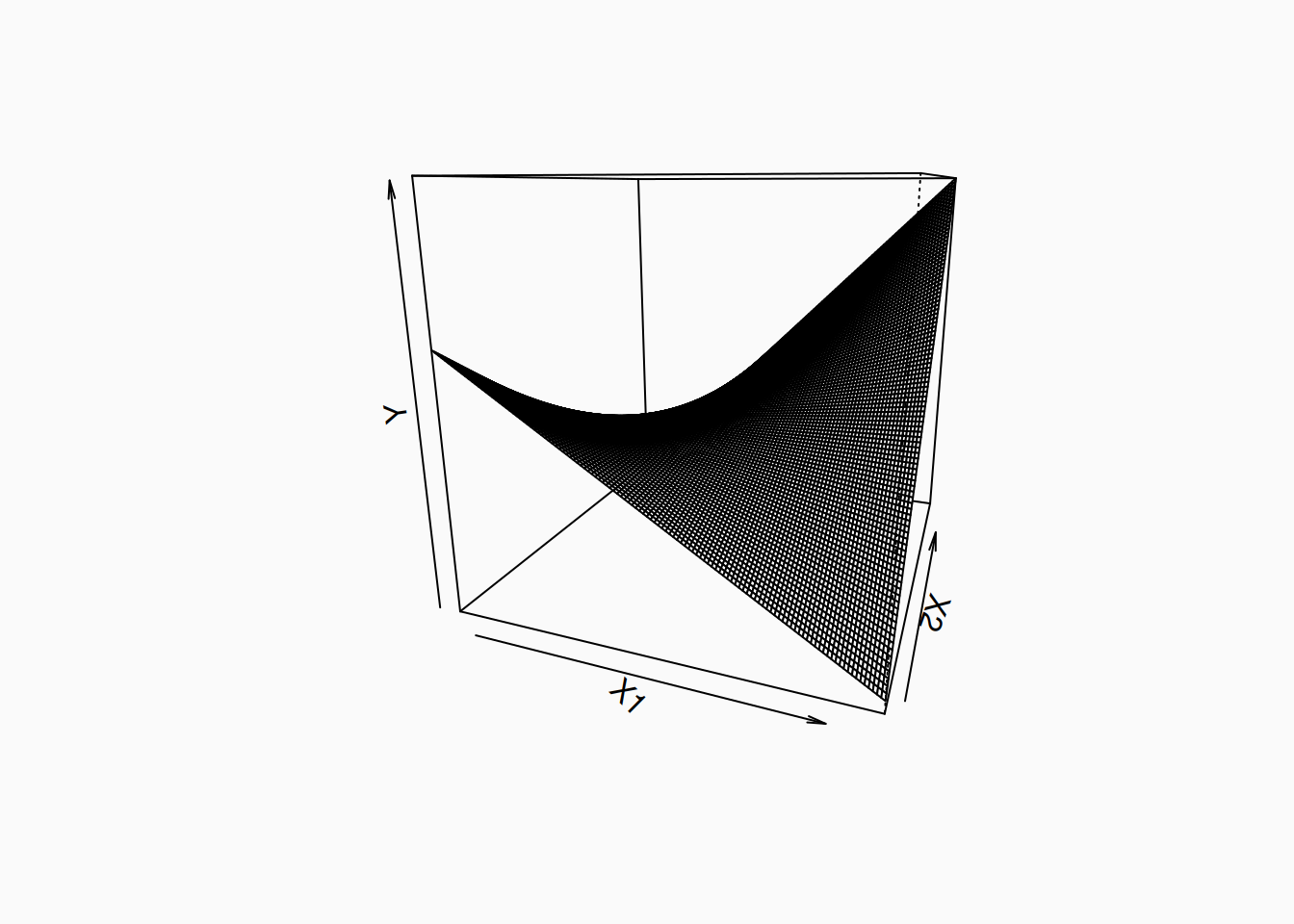
Obviously there’s a curved shape here in three dimensions, which is hard to describe. One approach is to think about what the slope of \(X_1\) is, when \(X_2\) takes different values. To do this, we can set \(X_2\) to particular values in the equation above, and then simplify the equation:
- If \(X_2 = 0\), then \(Y = 12 + 2X_1\):
- This means that a one-unit change in \(X_1\) predicts a two-unit change in \(Y\).
- If \(X_2 = 1\), then \(Y = 4X_1\):
- Now a one-unit change in \(X_1\) predicts a four-unit change in \(Y\).
- If \(X_2 = 2\), then \(Y = 20 + 6X_1\):
- A one-unit change in \(X_1\) predicts a six-unit change in \(Y\).
- If \(X_2 = -1\), then \(Y = 8\): Changes in \(X_1\) don’t affect \(Y\). This is not visually obvious in the graph (3D graphs suck).
- If \(X_2 = -2\), then \(Y = 4 - 2X_1\): A one-unit change in \(X_1\) predicts a negative-two change in \(Y\).
So the “slope” of \(X_1\) depends on \(X_2\), as we can see in the graph above: when \(X_2\) is higher (toward the back) the surface slopes upward from left-to-right; when \(X_1\) is lower (toward the front), the surface slopes downward from left-to-right. Note that we could also compute the slope of \(X_2\) given values of \(X_1\), which would give us a different perspective on the equivalent information.
General Linear Models
The simple/multiple regression models described so far only involve continuous numeric variables. However, with a little hoopla, the linear model can be extended to:
- Use categorical or ordinal independent (\(X\)) variables.
- Represent “curved” (polynomial) relationships.
- Represent categorical dependent variables (classification).
- Use different error distributions—not always the normal distribution!
- Represent multiple dependent variables (\(\{Y_1, Y_2, Y_3, \ldots\}\)).
- Incorporate multiple sources of random error, to account for “sticky data.”
In this chapter, I’ll go over the first two of these; #3 and #4 will be discussed in the Normal Assumptions chapter; #5 and #6 are discussed in the Statistical Tests appendix.
The all-encompassing linear model that can incorporate all these possibilities is called the General Linear Model (GLM).
Categorical Independent Variables
How can a “linear” model represent categorical data? For a binary variable its straightforward: just pick two arbitrary numbers to represent each category. By convention we assign one category 0, and the other 1; the means that a “one-unit change” in the regression “slope” means changing from 0\(\rightarrow\)1. We say that the categories are coded as 0 and 1. Usually, we assign a “baseline,” “reference,” or “control” category to 0; however, the choice is unimportant and often arbitrary.
Note that the mathematical model doesn’t “know” that there are no numbers in between, or beyond, zero and one, but we know, and should keep it mind.
To represent two or more categories, we cannot just add more codes: e.g., 0, 1, 2, 3. If we did this, the model would be assuming that the categories fall on an ordered continuum and that the “distance” between each category is the same. This is not appropriate for a categorical variable. Instead, the answer is to represent each categorical variable with more than one “coded” \(X\) variable. In fact, if our variable has \(k\) levels, we will need \(k - 1\) coded variables: to represent three categorical variables, we need two \(X\); for four categories, we need three \(X\); etc. Don’t worry, your statistical software will do this coding stuff for you, but it’s important to understand it if you want to be able to interpret your results.
There are a number of different ways categorical-variables can be coded. Here, I will just show you the most common scheme, called “treatment” or dummy coding; you can learn other coding schemes in the Statistical Tests appendix. To represent an Instrument variable with four levels—\(\{Voice, Guitar, Drums, Other\}\)—we’d need three coded \(X\) variables. The dummy coding would look like this:
| \(X_{guitar}\) | \(X_{drums}\) | \(X_{other}\) | |
|---|---|---|---|
| \(Voice\) | 0 | 0 | 0 |
| \(Guitar\) | 1 | 0 | 0 |
| \(Drums\) | 0 | 1 | 0 |
| \(Other\) | 0 | 0 | 1 |
Notice that the \(Voice\) level doesn’t get its own \(X\) variable: We say that the \(Voice\) level has been set as the “intercept” level, because it will simply go with the intercept \(\beta_0\) term. (We could choose any of the other levels to be the intercept instead.) To represent one categorical variable with four levels, our linear equation would actually look like this, with three coded variables:
\[ Y = \beta_0 + \beta_1X_{Guitar} + \beta_2X_{Drums} + \beta_3X_{Other} + \epsilon \]
How does this work? If a data point is sampled from the \(Guitar\) category, then \(X_{Guitar} = 1\), and the other coded \(X\) variables are \(0\).
\[ Y = \beta_0 + \beta_1 * 1 + \beta_2 * 0 + \beta_3 * 0 = \beta_0 + \beta_1 \]
It would work the same for either \(Drums\) or \(Other\). However, if you’re in the \(Voice\) category—the intercept category—, all three coded \(X\) variables are set to \(0\), so we get:
\[ Y = \beta_0 + \beta_1 * 0 + \beta_2 * 0 + \beta_3 * 0 = \beta_0 \]
Just the intercept is left over.
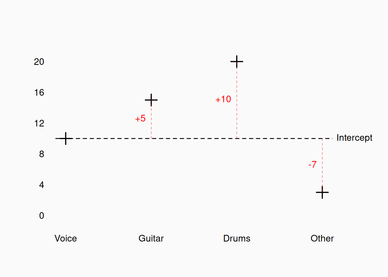
What does this look like with actual numbers? Let’s fill some in:
| Coefficient | Category | |
|---|---|---|
| \(\beta_0\) | 10 | Voice |
| \(\beta_1\) | 5 | Guitar |
| \(\beta_2\) | 10 | Drums |
| \(\beta_3\) | -7 | Other |
So, what would \(Y\) be in each category?
- \(Voice\): \(Y = \beta_0 + 0 + 0 + 0 = 10\)
- \(Guitar\): \(Y = \beta_0 + \beta_1 + 0 + 0 = 15\)
- \(Drums\): \(Y = \beta_0 + 0 + \beta_2 + 0 = 20\)
- \(Other\): \(Y = \beta_0 + 0 + 0 + \beta_3 = 3\)
Each coefficient represents the difference between that level and the intercept level:
Curved relationships
There are several ways that “curved” relationships can be incorporated into linear models. One basic approach is to simply apply a (relevant) transformation to a variable. For example, imagine that we want to use \(F_0\) frequency as a linear predictor of something else, like perceived energy in a vocal. If we gathered some data, we might see a relationship like this:
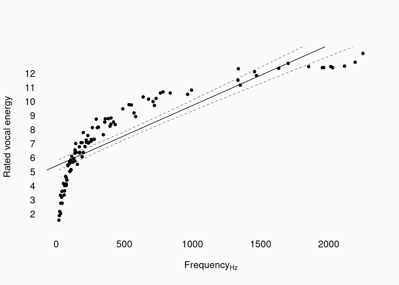
Clearly there is a curved relationship here and the linear regression line (which I’ve drawn) is not a great model of this data. But wait—we know that humans perceive changes in frequency rationally, right? For example, an octave is 2:1 ratio and a perfect fifth is a 3:2 ratio, etc. If we transform our frequency variable by taking the log, we create a new variable where human perception of intervals is linear. (We’ll use a base-2 log, so the units of our new variable correspond to octaves.)
Here is the same data, with the log-transformed frequency:
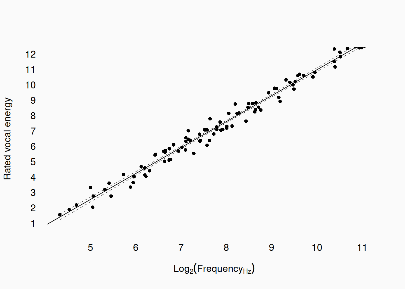
Ah! It appears that the relationship between log-frequency and the vocal rating is almost perfectly linear. We can even transform this straight regression line back into our original frequency space, if we really want to:
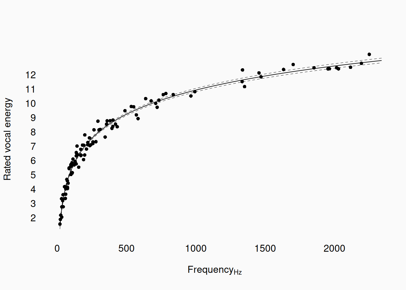
This line is curved in frequency space, but linear in log-frequency space.
Frequency is an example of a common music-research variable that we expect, a priori, to be “log-linear.” When planning our inquiries and analyses, you should generally transform variables a priori (before analysis), if it makes theoretical sense to in the context of your inquiry. However, you might sometimes realize the need to apply some sort of transform post hoc—especially in exploratory research. If, during your descriptive visualization, you notice some apparently curved relationships between variables, you could try various transforms of your variables to see if any result in a more linear fit: e.g., taking a logarithm or exponentiating the variable (\(X^2\) or \(2^X\)). If you can find a way of making the relationships linear, then all the power of linear models is put at your disposal! Of course, any transformations that you decide on post hoc should be described as such.
Polynomial Regression
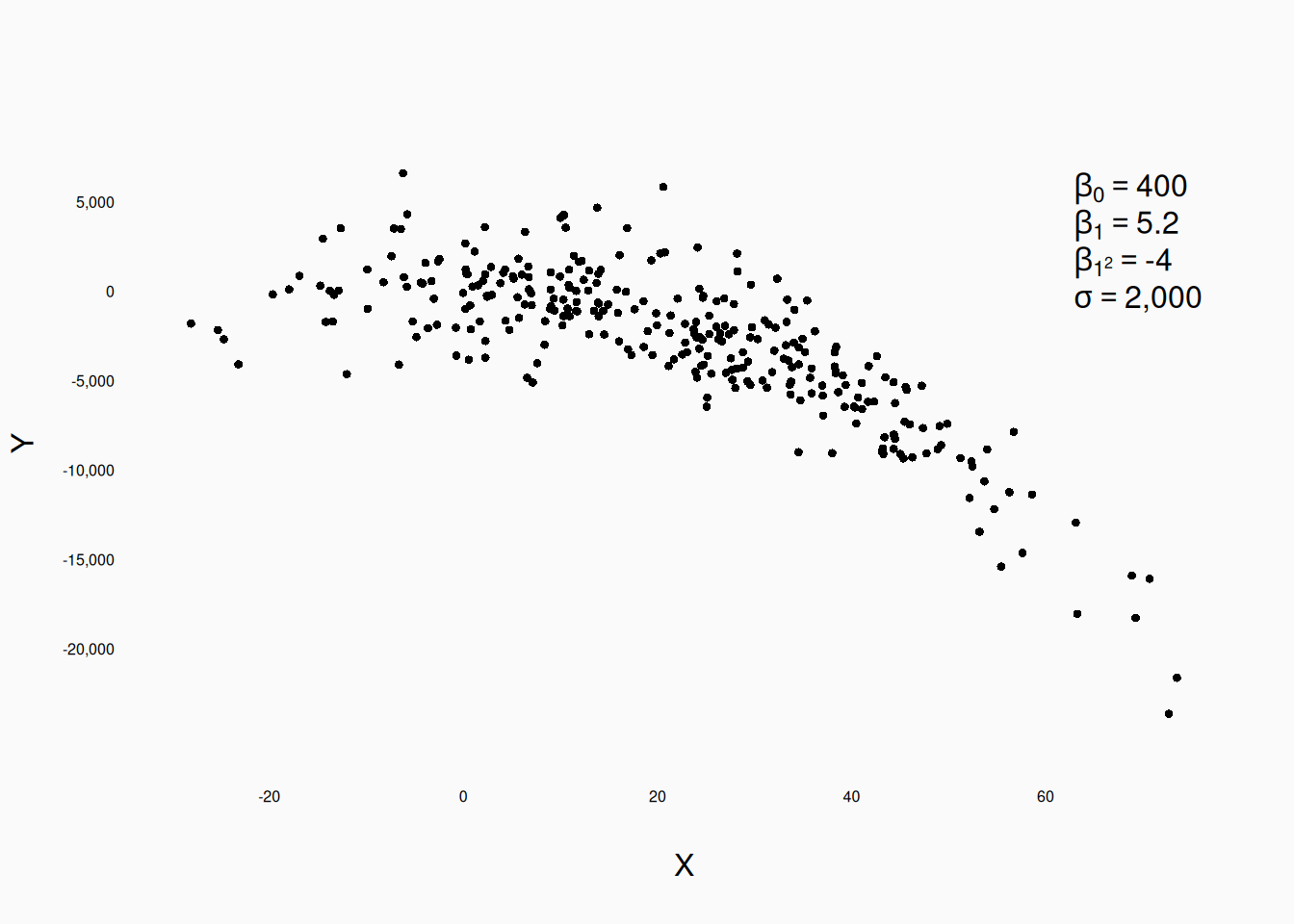
There is another, more general, way to incorporate curved relationships into linear models: polynomial regression. This involves, for a given numeric independent variable, adding additional exponentiation terms to the model, each with their own \(\beta\) coefficient. For example, if we are looking at the relationship between a dependent variable \(Y\) and an independent variable \(X\), we might include a quadratic \(X\) term, like this:
\[ Y = \beta_0 + \beta_1X + \beta_{1^2}X^2 + \epsilon \]
\[ \epsilon \sim \mathbb{N}(0, \sigma) \]
Such a model can generate data like this:
We can extend this to higher-order polynomials:
\[ Y = \beta_0 + \beta_1X + \beta_{1^2}X^2 + \beta_{1^3}X^3 + \beta_{1^4}X^4 + \epsilon \]
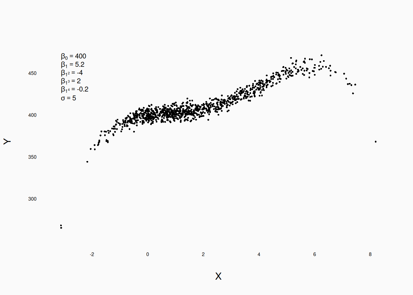
Note: For any of these higher-order terms, it is important to include all lower order terms: i.e., if you include \(X_{1^2}\), you must also include \(X_1\). This allows the multiple-regression algorithm to calculate “partial” \(b\) coefficients, for each term.
There is a danger in polynomial regression: a sufficiently high-degree polynomial curve can always “fit” your data. For example, here is some data generated by a purely linear model, with it’s “true” regression line overlaid in blue:
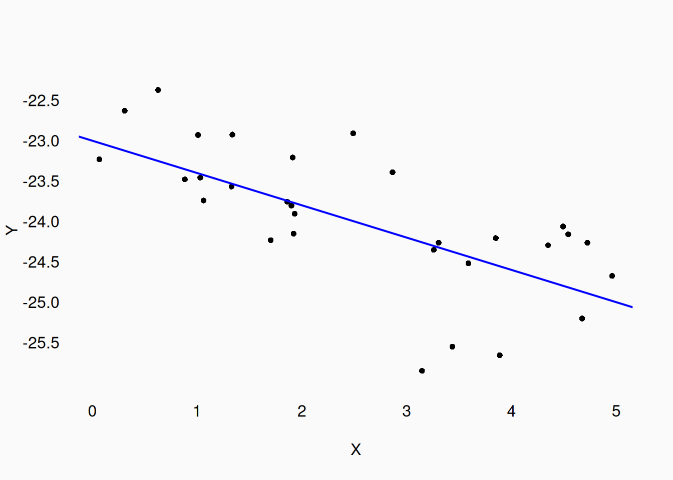
Here is how a 5th-order polynomial regression model fits the data (in red):
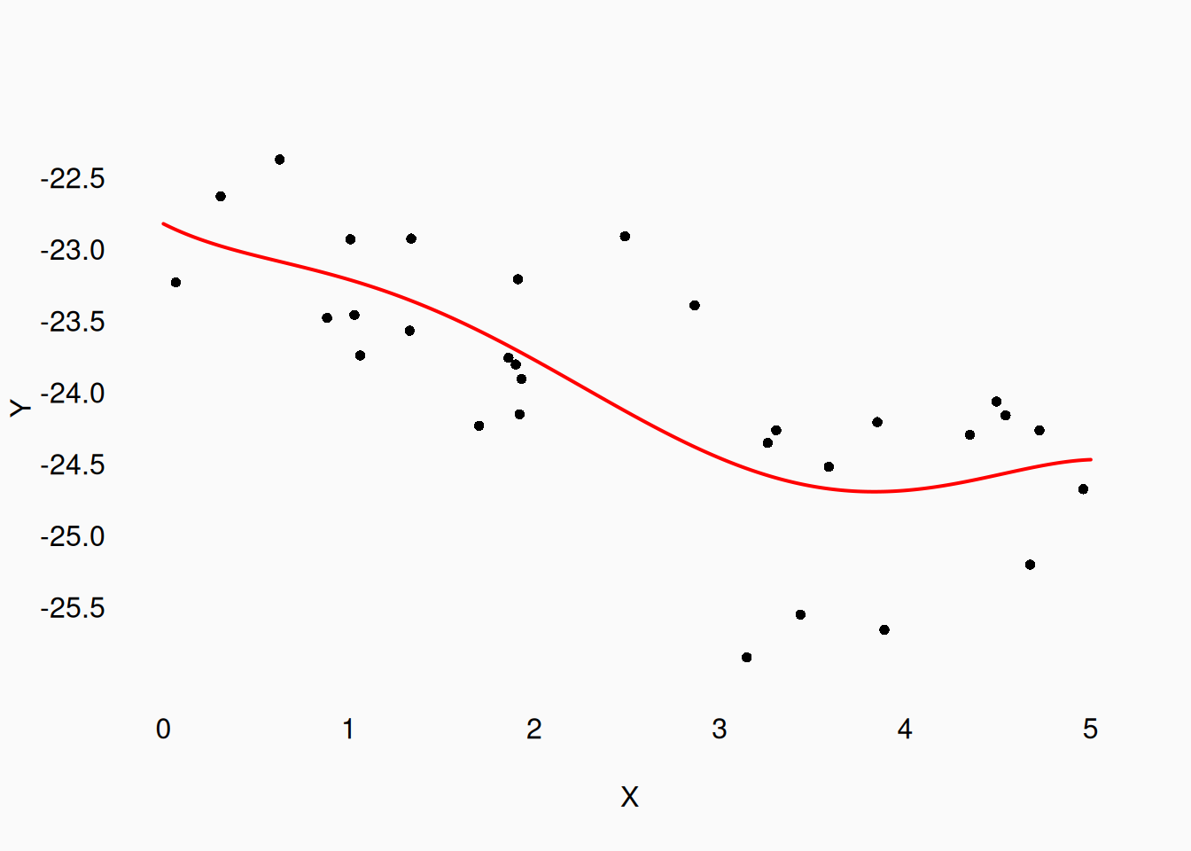
Pretty plausible match to the data right? What about a 10th-order polynomial (in green)?
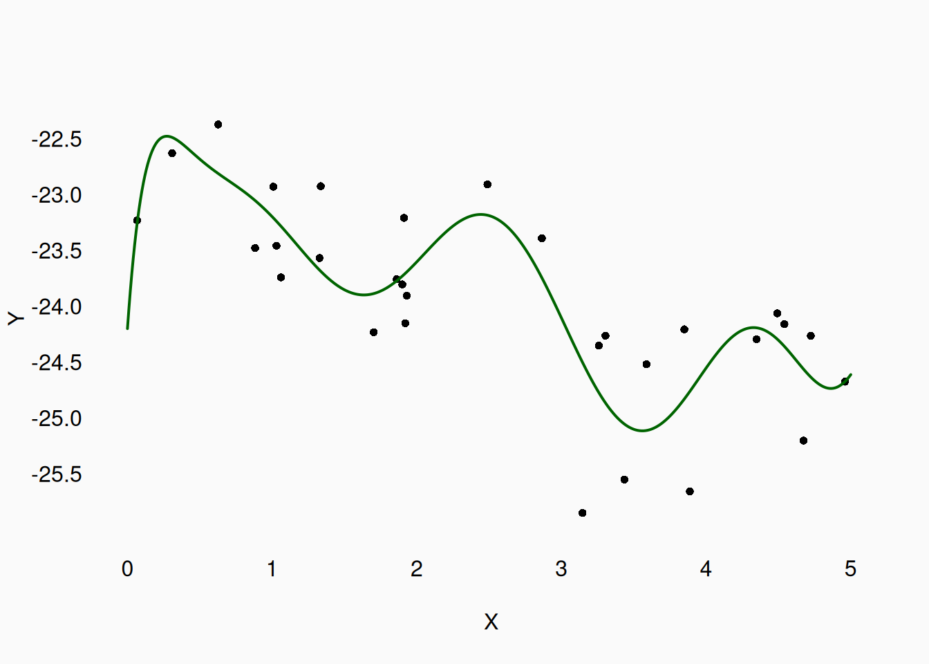
This curvy line follows the data very closely. However, in this case we know that the true population data generator was a just a straight line (blue line above). The green (10th-order) and red (5th-order) lines might seem like good descriptions of the data, but they are misleading any inferences we would make. They are over-fitting the data. Given random data, it can often appear that there are “curves” in the data that aren’t really there at all. A simple “straight line” might not seem like a good fit, when in fact it is. The lesson is this: don’t start looking for curved lines unless you have a real good reason to.
Purely linear models can seem boring and simplistic, whereas polynomial models might seem cooler and fancier. But we must remain skeptical, especially of models that are highly prone to over-fitting data. Generally, using non-linear approaches without good, a priori/theoretical reasons, will be looked on with skepticism. In many ways, linearity is a default assumption: unless there is strong evidence—or better yet, strong theory—to the contrary, assume linear models!
For example, \(y = x^2\) or \(y = \frac{x}{1+x}\).↩︎
Note we use “\(s\)” because it is analogous to the sample standard deviation.↩︎
This happens because the covariance is multiplied by \(4\) but the variance of \(X\) is multiplied by \(4^2\), so the overall \(\beta\) is divided by \(4\).↩︎
The standardized \(b\) is the same as the covariance of \(X\) and \(Y\) divided by the standard deviation of \(X\): \(b* = \frac{s_{XY}}{s_X}\).↩︎
That’s upper-case sigma and upper-case S.↩︎
You can also calculate the equivalent “partial” correlation coefficients, but this is not terribly common.↩︎