26 Samples
(Modified on 2026-08-11)
4,263 words
Typically, the constructs we are interested in relate to widespread (musical) activities. However, when we measure a variable, we only observe a finite sample of the possible observations that we could observe. Any sample is an incomplete representation of the true underlying construct. To what extent can analysis based on a sample be generalized to the construct in general? This is the question of external validity.
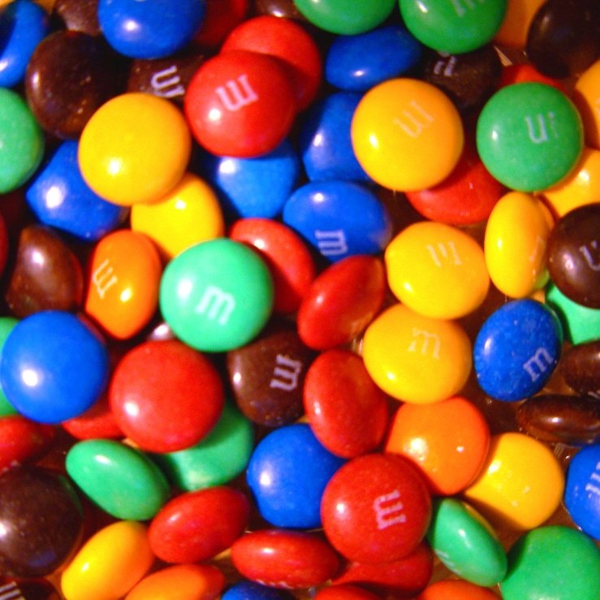
Imagine that you land a job working at Mars, Inc. quality control. You are told that 20% of M&Ms produced at your factory should be green; no more, no less.
How can you check if a day’s batch of M&Ms (10 million candies) has the correct proportion of green candies? Obviously, you can’t count them all! The best you can do is estimate the proportion of the batch which is green. You stick a cup into the batch and scoop out some M&Ms. You count them, and find that there are 111 in total and 25 are green—22.5%. Based on this, you estimate that roughly 22.5% (2.25 million) of the whole batch is green. This (hopefully) makes intuitive sense, but why does it work? And how can it go wrong?
The “population”
In statistics, there is a common metaphor used to think about sampling: the population. The population is something we postulate: a specific set of all possible relevant data that could by hypothetically observed. Each sample then is a subset of this (usually much larger) population.
\(Sample \subset Population\)
The goal of sampling is to enable us to make accurate claims about the population, even though we have only examined a subset of that population. In the example above, the full batch of (\(10^7\)) M&Ms is the population. The scoop of M&Ms is a sample. We inspect the sample (scoop) to make inferences about the population (batch).
A batch of M&Ms is a very straightforward population. However, in real research, identifying the precise population that you want to make claims about can require careful thought. For example, you might want to make claims about the population of (human) music listeners. But do you want to make claims about…
- All the world’s living people?
- All the world’s living adult people?
- All the world’s people, living and deceased?
- All the world’s living people, plus those who will be born in the next 20 years?
- All people who enjoy listening to music?
- All Western-enculturated people?
- All clarinet players?
Not just people
Lots of sampling theory and methodology is focused on sampling from human populations. However, a research “population” is a set of observations—not necessarily a set of people. For example, we might also want to make claims about…
- The population of M&Ms produced between January 1 2013 and December 31 2020.
- The population of notes in compositions by W.A. Mozart.
- The population of tracks available on Spotify.
- The population of emotional responses to music.
- The population of drum beats in the music of Metallica.
Defining a population
Defining your population can be just as difficult as other research definitions. There are always details to consider:
- “All Western-enculturated people”…
- Does that include children?
- What about deaf people?
- How long do you have to live in the West to be “enculturated” there?
- What is part of the “West”?
- “The population of M&Ms”…
- Any kind of M&M, or only plain M&Ms?
- The M&Ms that exist right now, or all the M&Ms that were ever made?
- “The population of notes in a compositions by W.A. Mozart”…
- Which compositions count? Only ones he published during is life time?
- Do grace notes or ossia staves count?
- Are tied notes counted?
- “The population of tracks available on Spotify”…
- Available when?
- Available to who?
- In which countries?
- “The population of drum beats in the music of Metallica”…
- In recordings only? Or do live performances or private jam sessions count?
- Is this only past releases, or does it include future work?
- If Lars Ulrich is playing with Kirk Hammett, but the rest of the band isn’t there, does that count as “Metallica”?
- If they cancel a gig due to bad weather, does the music that they would have played that night count?
- In recordings only? Or do live performances or private jam sessions count?
In research, all we ever actually work with is samples, and we never really know what our samples represent. We might want to target a specific population (of people or data), but our sampling strategies might fall short. We must then adopt a bottom-up thought process: Given a sample, what population can we generalize about? What does our sample actually “represent”? Most importantly, does it represent the cases we actually care about?
It’s up to us to judge and/or argue what a sample represents—and what valid conclusions can be generalized to what population. You might claim that your sample represents music listening in general; A reviewer might think the results only apply to young people, or Westerners, or educated Westerners, etc. Couching the generalizability of your results is a good opportunity to forestall critiques. It is common to have some disclaimers in the conclusion of a paper noting, among other things, what population the sample may or may not represent.
Sampling Error
As we know, each measured value has error—a difference between the “true” level and the measured level. Sampling introduces another perspective on error; how variation in the sample differs from variation in the “true” construct. As with specific measurement errors, we can think of two types of sampling error: random and systematic sampling error. Modeling random sampling error is the core goal of statistical analysis. Systematic sampling errors—sampling bias—cannot generally be “fixed” in analysis, but needs to be avoided in the sampling process.
Above, we estimated that 22.5% M&Ms of a batch of ten million are green. Why is this estimate plausible? Why would it be a valid claim?
In order to generalize from sample to population, we need to confidently argue that the sample “represents” the population. The key to making this argument is showing that our sampling procedure is uncorrelated with our variable(s) of interest (e.g., M&M color). For example, if our sampling procedure is to “scoop a cup of M&Ms from within arms reach,” we must ask if the variable “within arms reach” is correlated with the variable “color.” If not, then the scoop should be an unbiased sample of the population. However, what if the red food coloring in M&Ms is slightly heavier than the other food colorings? If so, the red M&Ms might tend to sink to the bottom and thus the variable “within arms reach” would actually be negatively correlated with the color red. As a result, any sample we took this way would be biased towards the other colors, including green. The resulting sample would not be representative of the population—there would be systematic sampling error.
Let’s consider a more musical example. Imagine that we want to compare the contributions of white and black musicians to American popular music in the 1960s and 1970s. We could randomly sample 1,000 songs which appeared on Billboard charts between January 1960 and December 1979, and look up the songwriting and performer credits for each song on Wikipedia. We might analyze the data and conclude that, in this period, 11% of hit song writers and 9% of studio musicians were black. What could be the problem with this claim? Well, during this era, black musicians in the United States were less likely to be credited for their performances and songwriting contributions than white musicians. In other words, the variable “race” was correlated with the variable “credit.” Thus, the sample of contributor names is biased against black musicians, and our conclusions don’t actually match the reality of the population.
Correlation with other variables
Valid sampling schemes have no correlation with the research variables that interest us. However, if the sampling scheme correlates with other variables—which are irrelevant to our work—our sampling may still be valid. This means, that sometimes something that seems like it’d be a terrible, unrepresentative, sample, could actually be valid. For example, imagine that you wanted to study the relationship between mode (major, minor, etc.) and emotional expression. To pursue this study you download a large, random sample of music from the internet—but due to bandwidth problems, only relatively short songs (less than four minutes) successfully download. So your sample is systematically biased towards shorter music…but would that matter? It seems unlikely that the relationship between mode and emotion would depend on the length of songs (perhaps you disagree?). So, the variable “song length” is an irrelevant covariate, and it doesn’t matter if our sampling is biased based on song length.
Let’s consider a more general example. Much of the foundational research about human physiology and psychology done in the 20th century was conducted using Western participants, especially (white) college students. Obviously, Westerners are not representative of humans in general. However, we are all humans, and basic human physiology doesn’t really differ that much around the world. If we are studying things like the frequency response of the auditory system, comparing people’s reaction times to auditory vs visual stimuli, or how precisely people can localize sound sources in space, it is not unreasonable to think that all human populations would have similar abilities. Why would we think that white people could hear higher/lower frequencies, or react faster/slower, than other people? The point is, that even an obviously unrepresentative sample in some respects, might still allow us to generalize about specific variables.
Of course, this doesn’t mean that we can ignore the problem of published research over relying on samples of Western college students as participants. Most human behaviors are influenced by culture in some way, which means that we definitely cannot generalize from one culture to others. Even some “basic” psychoacoustic abilities are (surprisingly) influenced by culture—for example, people who grow up in dense forested environments can develop better spatial perception abilities, because they frequently hear sounds above them. Another concern is that most physiological abilities are age dependent—just because college students can hear \(20_{kHz}\) doesn’t mean that most (older) adults can!
Sampling Fallacies
Many, many cognitive fallacies and scientific errors can be attributed to sampling bias. We observe something and over (or under) generalize, because our sample doesn’t actually represent a population we care about. There are two main problems to watch out for: 1) that the data selects itself and 2) that the researcher selects the data.
People often complain that “pop music these days” is terrible. Why? We are surrounded by varied examples of contemporary pop (most bad, some good) every day. However, when we sample music from 10, 20, or 200 years ago, only the best music is remembered, or even preserved. A typical sample of (Western) music from two centuries ago only includes music by a handful of the greatest composers who ever lived—their numerous mediocre contemporaries are forgotten. Similarly, a classic rock radio station exclusively plays the best music of the 1960s and 1970s, never playing worse music from the same era. Even our personal memories tend to work this way—we simply don’t remember the boring uninteresting things we were exposed to! As a result, our samples of older music tend to be biased towards “good” music, while our sample of current music has no such bias. This is an example of survivorship bias: The data has been pre-filtered based on relevant variables (in this case, quality)—we are only sampling data that “survived” the screening.
A related problem is volunteer bias or response bias: in this case, the data (e.g., human participants) chooses to be sampled, and the choice might be influenced by relevant variables. If you send out a 1000 surveys (via email) only a small percentage (maybe 10%) of people will bother filling it out for you. This is not inherently a problem. The problem is that this 10% is not representative of the whole group—they will tend to be people who are more considerate and diligent in general, or people who happen to have strong opinions or interest in the topic of your survey. If variables like “is diligent” and “has strong opinions about the research topic” correlate with our research variables (they very likely do), bias is introduced. A similar, but opposing effect, is attrition bias, where a non-representative group of data/participants “drop out” of an ongoing study. For example, educational research which tries to follow groups of children over the course of several years will have some percentage of the families drop out of the study each year. In many cases, families that “drop out” have common attributes (like less money, or interest in education) that those that stick in, so the students that are left in the sample at the end are not representative of the whole group.
If you select data based on relevant variables, it may also be biased, consciously or unconsciously. Our attention, as people and researchers, tends to be drawn to the most unusual, interesting, or prominent phenomena we encounter—an effect called salience bias. The most common example of data biased by salience is anecdotes: An unusual or interesting instance that grabs our attention, but which is (probably) not generalizable. Researchers might, for example, gather data by standing in a public area and interviewing people as they pass. Bias can be introduced because the researcher may be attracted to approach certain people and not others. For example, a researcher may be more likely to stop someone who is smiling; This will potentially bias the sample toward “friendly” people. Also, curious people may hang around hoping that the researcher will ask them to contribute (volunteer bias).
An even worse issue is that we tend to notice things more that confirm our expectations: confirmation bias. Any sampling procedure that gives the experimenter a lot of control can be biased towards data that confirms their hypotheses. For example, imagine that a researcher hypothesizes that Lars Ulrich (Metallica) is the worst metal drummer. They sample a bunch of Ulrich’s playing from the Black Album—an album often criticized for boring drum-beat choices. For comparison, they sample drumming by David Lombardo (Slayer), who is often regarded as an excellent metal drummer. What’s the problem here? Their sampling choices were based on the quality of drumming, which is the variable they are interested in. The researcher has assured that their conclusion is true in their sample, but this is a poor argument that the conclusion is true in general. To do this properly, we’d need a random sample of Ulrich’s drumming and a random sample of other metal drumming, for comparison.
In its most extreme form, confirmation bias can take the form of “cherry picking”—consciously, or unconsciously picking out specific examples that support your theory. Reviewers are very wary of cherry picking!
Sampling Methods
To avoid sampling bias, the core technique is randomization: If we select data randomly, neither we nor the data control what is sampled. If done correctly, this assures that sampling error is random (as opposed to systematic) and thus unbiased. The key, again, is that no variable of interest should correlate with the sampling procedure, and randomization is our best hope to achieve this. Of course, “randomization” doesn’t just happen; we need to have some procedure for how we randomly sample, and we want to make sure this procedure doesn’t correlate with any variables either.
To represent a population, the ideal approach is to sample any possible element from the population with equal probability: this is called simple random sampling.
Suppose we have a video recording of an audience listening to a concert of music by the composers Schoenberg and Ravel. The video camera allows us to see all 150 audience members and the recording lasts 40 minutes. Before accessing this video, we hypothesized that members of the audience would “fidget” more when listening to Schoenberg compared with Ravel. Counting the fidgets for each audience member over the entire recording would require too much work. To simplify the problem, we might randomly select 25 of the 150 audience members. In addition, instead of coding data for the entire video, we might count the number of fidgets during twenty randomly selected 10-second segments: ten 10-second segments from the Schoenberg work and ten 10-second segments from the Ravel. Here we are randomly sampling from the total visible audience, and also randomly sampling from the total length of the video recording. If any audience member, and any 10-second segment, is equally likely to be sampled, then we can be reasonably confident that our sample will be representative. To do this, we might assign each audience member a number (from 1 to 150) and use a random number generator to select 25 numbers; similarly, we can use a random number generator to sample 500 numbers (20 segments times 25 participants) from the range 1 to 2,390 (40-minutes is 2,400 seconds), to identify the start of our ten-second sample segments.
Sampling Strategies
In practice, actually sampling randomly can be difficult, especially for field work or any case where a researcher has to pick samples. In these cases, it is important to apply a systematic sampling scheme to force yourself to make random choices. As always, you need a system that is independent (uncorrelated) with the variable of interest.
Say we’d like to distribute questionnaires to people leaving a concert hall. One approach would be to distribute the questionnaires to the first 50 people leaving the concert hall. Notice, however, that this might bias our sample towards people who are in a hurry, or people who didn’t like the concert and are eager to leave. Even if we attempt to sample people at random, our sample might be affected by salience bias, volunteer bias, confirmation bias, etc. One solution to these problems would be to hand-out our survey to every tenth person as they exit from the concert hall. It’s unlikely that the variable “10th person to exit” is correlated with anything meaningful. Similarly, if you are sampling notes in a score, you could sample every 50th note.
You might also sample systematically based on some other random, uncorrelated criteria. For example, you could look at a group of people’s calendar day of birth, or the last digit in their phone number. By following a (simple) system, your sampling decisions are no longer (potentially) biased by other factors.
A new approach to enforcing randomness “in the field,” is actually using an external randomization app; I’ve noticed that airport security personnel now have a randomization app on their phone which tells them when to randomly search people. This avoids various biases that can crop up if we allow personnel to choose who to search.
Stratified Samples
Unfortunately, simple random sampling is often insufficient to sample all the different variable levels/conditions you are interested in. Why? Let’s say you are interested in how gender and sexuality correlate with musical taste. Even if you randomly sample 50 people, you might only get two or three homosexual participants—which is insufficient to make any useful conclusions. An alternative approach is, thus, stratified sampling: sampling equally from groups based on one or more variables. We might for example, aim to sample 15 each of straight women, gay women, straight men, and gay men. We might do stratified sampling based on any variable which we want to control, or are interested in studying: demographic information (gender, age, race, ethnicity), income, decade of album release, instruments, musical experience, etc.
In a recent paper, Beach Clark and I (2024) hypothesized changes in the “tempo stability” of recorded music over the last half century. Our main independent variable was the year of a track’s release; we also considered genre to be an important covariate to consider. To make sure we had a good representation of tracks across various combinations of these two variables, we employed a stratified sampling scheme. Specifically, we sampled 100 tracks from each year between 1920 and 2020 for each of seven genres: rock, country, blues, jazz, classical, hip-hop, and EDM. Of course, there were no hip-hop or EDM tracks from the 1930s (actually there were, because of errors in the Spotify data), so our year and genre variables were not fully crossed in the sample. The data and analyses can be visualized here.
A compromise between simple-random and stratified sampling is quota sampling: sampling from subgroups proportionally to their prevalence in the population. Suppose that we find that 55% of American musicians are primarily guitarists, 30% are primarily pianists, 12% are flautists, 9% trumpeters, 8% violinists, etc. In quota sampling, we would aim to sample to match these proportions—for example, 18 guitarists, 10 pianists, 4 flautists, 3 trumpeters, 2 violinists, etc.
Collister and Huron (2008) were interested in the intelligibility of vocal lyrics. They collected a sample of 78,000 words from lyrics, and found that 81% were monosyllabic, 16% were bisyllabic, and 2% were trisyllabic. In testing the intelligibility of individual words in a sung context, they employed the same proportions of monosyllabic, bisyllabic, and trisyllabic words. Similarly, if you want to sample 200 Americans, you might look up current demographic information for the country and sample different ethnic/racial groups in proportion: 72.4% White Americans (145 in sample), 12.6% Black Americans (25 in sample), etc. If you don’t apply quota sampling, it’s very likely that you’ll end up with, for example, an over representation of white guitarists in your samples.
Matched Samples
One final sampling strategy to consider is matched random sampling. Matched random sampling is a way of maximizing experimental control between two groups (or two levels of any variable) you want to compare. For example, if you are studying the differences between professional and amateur musicians, you’d like to isolate the professional/amateur variable as much as possible. You could start by randomly sampling professional musicians, then sample amateur musicians who “match” each professional. For example, you could match each amateur with a professional who plays the same instrument, or the same styles of music. You could also make sure matched pairs are the same age, gender, or any other criteria. You can also do matched sampling with other types of observations:
- If studying the difference between major- and minor-key music, we might pair a randomly selected work in the major mode with a randomly selected work by the same composer in the minor mode.
- When studying what makes a “hit song,” we might pair the top-10 hits from each year of the 21st century with the ten songs released by the same artists in the same year, but which never charted.
Convenience
Unfortunately, the number one factor that determines our sampling schemes is convenience. Why? Because research can only be done if it is practical.
- It is impractical to recruit participants drawn from all over the world.
- It is impractical to sample music which we don’t have access to.
- It is impractical to sample musical experiences in their natural environment (outside the lab).
In practice, we are often forced to work with whatever data we can get our hands on. For example, a sample of choral music might consist of all of the scores available in the School of Music score library. Similarly, we might stand on a street corner and ask whoever passes by to answer questions on a survey, or more often, share our experiments by posting links to our friends on social media. Convenience samples are nearly always biased in some way, but they are easy to assemble.
A lot of work with “big data” these days is driven by convenience samples: Datasets that have been assembled by somebody else and hosted online. Using these convenient datasets is not ideal, but is often a necessary evil. However, it is still important to consider how these datasets were themselves sampled, and what sort of data they contain. Only then can you (hope to) make strong claims using convenient data.
I recently reviewed a paper which relied on data sampled from the Spotify database. The paper was analyzing changes in several acoustic features that the Spotify dataset includes. On inspecting the dataset, I noticed that the sample included a number of non-musical tracks, including books on tape, comedy shows, podcasts, and dramatic performances. Evidently, the authors didn’t notice these non-musical examples and made no effort to exclude them, so their data analysis included the “danceability” metrics of A Song of Ice and Fire and the comedy of Tim Allen. The lesson: if you are going to use a convenient sample, inspect it closely! Learn what’s in it, and what’s not in it. All too often I see students using existing datasets without bothering to really understand what’s in them.
It is reasonable to rely on convenience samples for research, but it is not reasonable to assume that a convenience sample is representative of the entire world. Convenience sampling is a bad-word, but one we’ll see a lot. It is important in any study to make a clear statement of what the sampling procedure was, even if it is mainly one of convenience, and to identify the limitations of any sample with regard to the presumed population of interest.
Sample Size
Notice that in this entire reading, we have not discussed the size of our samples. As we will learn about and formalize in a later chapter, the larger a sample is the more likely it is that it will mimic the population it is drawn from, reducing the effect of random sampling error. However, the more insidious risk of systematic sampling error—where our sample doesn’t represent the population we think it does at all—is not affected by sample size. You can sample a huge amount of data, but if the sample is biased or problematic, it makes no difference. Conversely, a good sample, assembled from truly random, independent draws from the target population, can be used to make useful inferences with a surprisingly small amount of data. So, the take home message is 1) don’t assume that a large amount of data makes a good sample and 2) don’t assume that a small sample can’t be used to support valid conclusions.
Mantras
Always check the content of your samples, especially when relying on convenience samples. What observations are included in the sample? What observations are excluded from the sample? What observations are missing?
Anecdotes are, by their very nature, unrepresentative samples of reality. Anecdotes give us ideas and motivate us, but their value as evidence in an argument is basically nil.