52 Normal Assumptions
(Modified on 2026-08-11)
367 words
In all our practice examples, we keep assuming that error in our dependent variables is normally distributed. This is very common. Why? For one, the normal (Gaussian) distribution is simply well understood, easy to use, and closely connected to the fundamental statistical theories of least-squares and maximum likelihood. There is also plenty of evidence that the “Gaussian-centric” approach is quite robust to violations of the assumption.1
Still, even if the Gaussian approach is robust, it is better to use different approaches when appropriate. In some cases, data is clearly non-normal—for example, it’s bounded or discrete—and using alternate models/assumptions is warranted. Luckily, the Generalized Linear Model gives us two mechanisms for breaking out of the Gaussian world:
\[ Y = link(\beta_0 + \beta_1X_1 + \beta_2X_2 + \ldots + \beta_nX_n + \epsilon) \]
| Independent variable(s) | Error | Dependent variables |
|---|---|---|
| \(link(\beta_0 + \beta_kx_k +\) | \(\epsilon) =\) | \(y\) |
- \(\epsilon\): The error distribution
- a.k.a., loss/cost/error function.
- \(link(x)\): A “link function”
- a.k.a., activation function or output layer.
Non-normal error
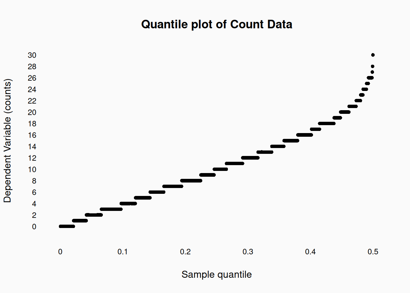
If our dependent variable is natural numbers (like counts, or ranks), a normal distribution isn’t really appropriate.
A normal distribution is continuous and unbounded; These numbers are discrete and have a lower bound at 0. We could still model this data using a normal distribution and it would probably not inflate our Type-1 error rate (much). However, we could do better by using an alternate model of the variable: in this case, we might use a Poisson distribution: \(\epsilon \sim \mathcal{Pois}(\hat{y})\). Here is an example of a Poisson regression, where the mean of the Poisson variable (the \(\lambda\) parameter) is modeled as a linear function of an independent variable:
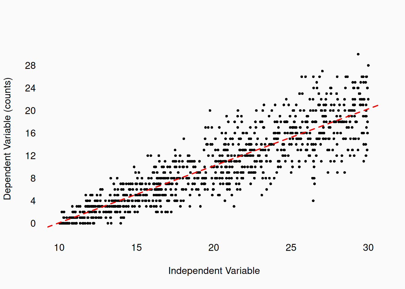
The result is not going to be terribly different than the result if we used a Gaussian model, most of the time, but sometimes the result might be different. It is our job to be skeptical of our data, analyses, and assumptions. In this case, it makes sense to be skeptical of an analysis that assumes normality: the Poisson regression is a better model of the data and just makes more sense. This makes for stronger rhetoric in our analysis.
Latent variables
Another way of incorporating non-normality into linear models is through a link (or activation) function. A link function is a non-linear transformation which we apply to our linear model:
\[ link(\beta_0 + \beta_kx_k + \epsilon) = \hat{y} \]
We can interpret this like this: we postulate that there is an “underlying” linear relationship—\(\beta_0 + \beta_kx_k + \epsilon = z\) in the data, but we don’t actually observe it directly. We call this a latent variable (in this case, labeled \(z\)). What we actually measure is a transformation of \(\hat{z}\): \(link(z) = \hat{y}\). This can produce an observed independent variable (\(\hat{y}\)) which is categorical, or ordinal, or anything else we want or need.
In many cases, we might argue that the latent variable represents the “true” research construct that interests us, while the link function and observed \(\hat{y}\) is “just” the result of our (imperfect) measurement protocol.
Likes
Consider the construct of “liking” music. We could model this construct as a one-dimensional, continuous (or at least ordinal), variable. You can like something a little, or a lot, or not at all, or anywhere in between. But what if, when it comes to measure or data, all we get is this?:

A binary, yes or no rating of “like.” We could postulate that users’ true “liking” of something is still a continuous variable, but we don’t observe that latent variable directly. Instead, users are forced to make a binary choice.2 We can then model the relationship between independent/predictor variables and the latent variable, even though we don’t observe it directly. For example, we might hypothesize that the latent “liking” variable has a linear relationship with a different independent variable, with normal error. If we could measure this, it might look something like this (a linear regression):
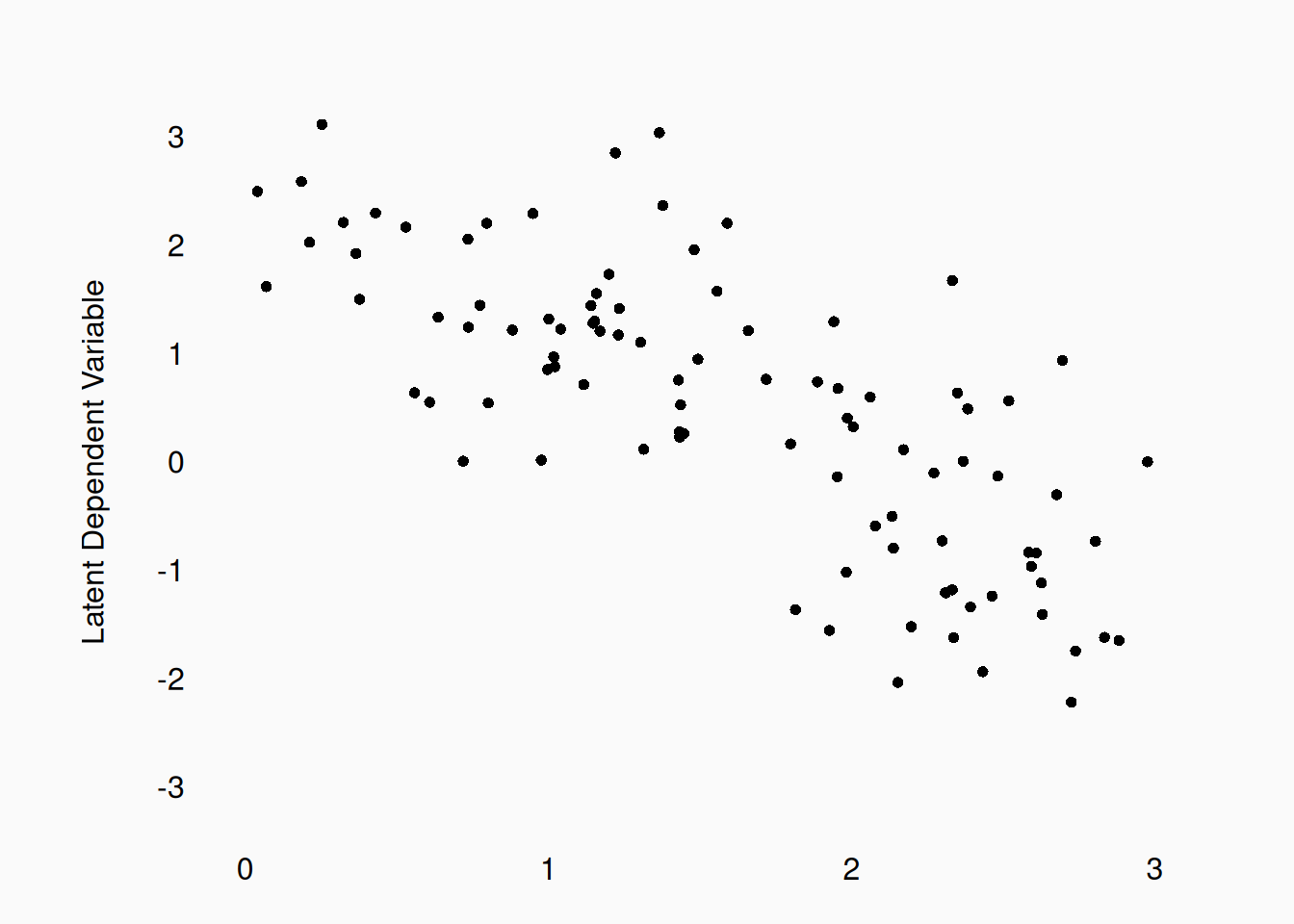
However, our actual dependent variable is only clicks. We might assume that users click “Like” when the latent variable is greater than zero:
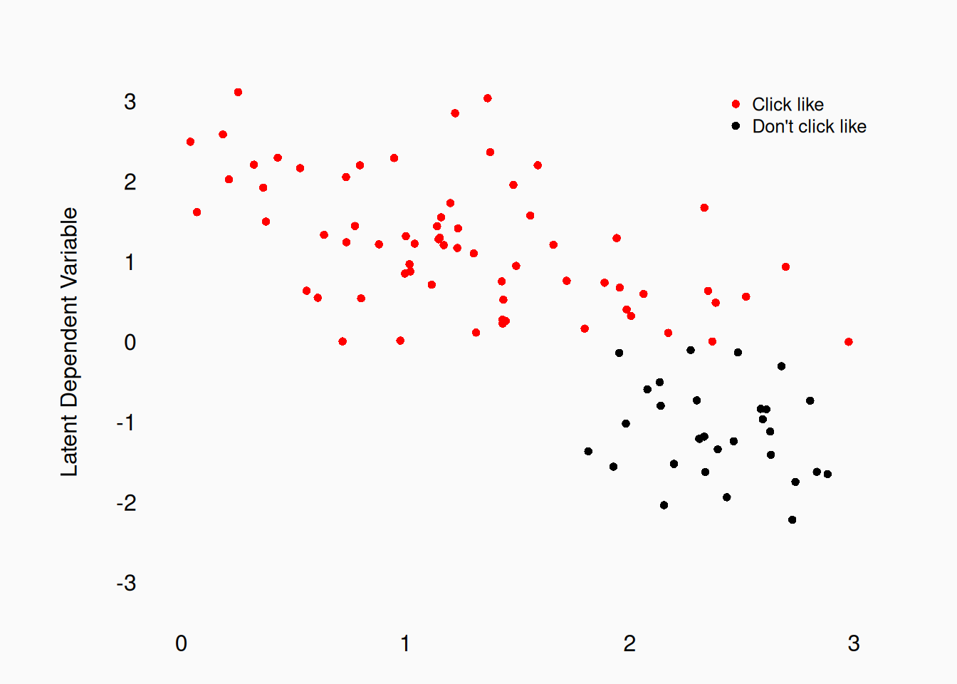
Of course, we never see the latent variable, so what we actually measure is this:
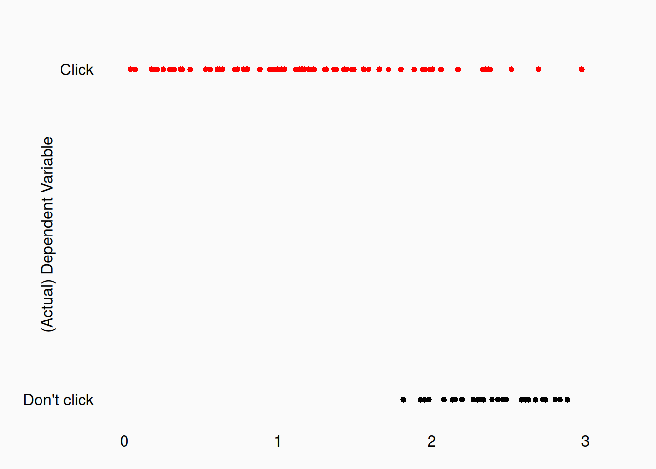
This approach, which assumes the error in the latent variable is normally distributed, is called probit regression. The link function here is the cumulative distribution function for the normal distribution, which gives us a probability value \(p\). The error function then is simply a binomial distribution \(\epsilon \sim \mathcal{Binom}(1, p)\). For these sorts of statistical models the least squares error model doesn’t make sense. However, we can still search for parameters that maximize the likelihood of the data we observe, and use this to estimate a probit-regression slope:
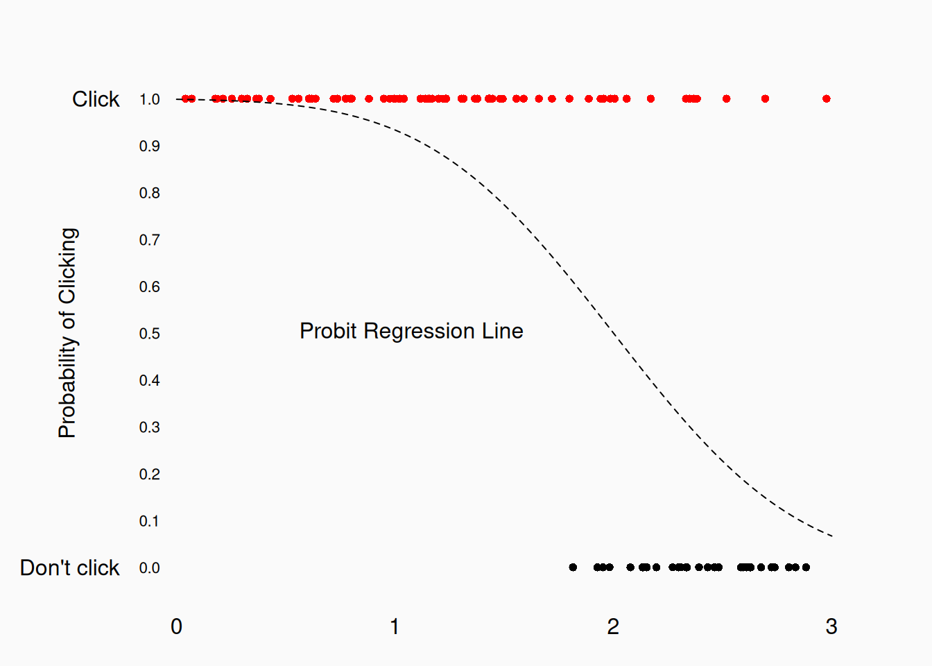
Unlike linear-regression scatter plots, the regression line here doesn’t represent the mean of a normal distribution. Instead, it represents the \(p\) of the binomial distribution, which we can interpret as the probability of clicking “Like.” The curve of this line is created by the probit link function.
Logistic Regression
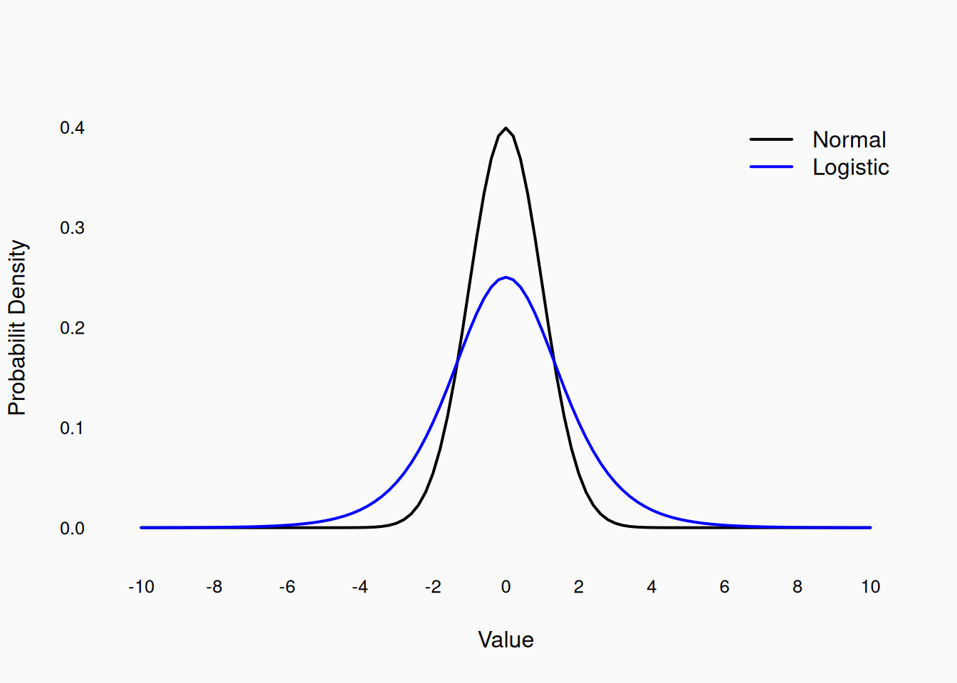
A similar, but much more common alternative to probit regression, is logistic regression. Logistic regression is the exact same idea as probit regression, except that we assume the latent variable’s error follows the logistic distribution, not the normal distribution. The logistic distribution is another “bell-shaped” distribution, but not the same as the normal (Gaussian) bell:
Here is an example of a linear scatter plot of a latent variable with a logistic error distribution:
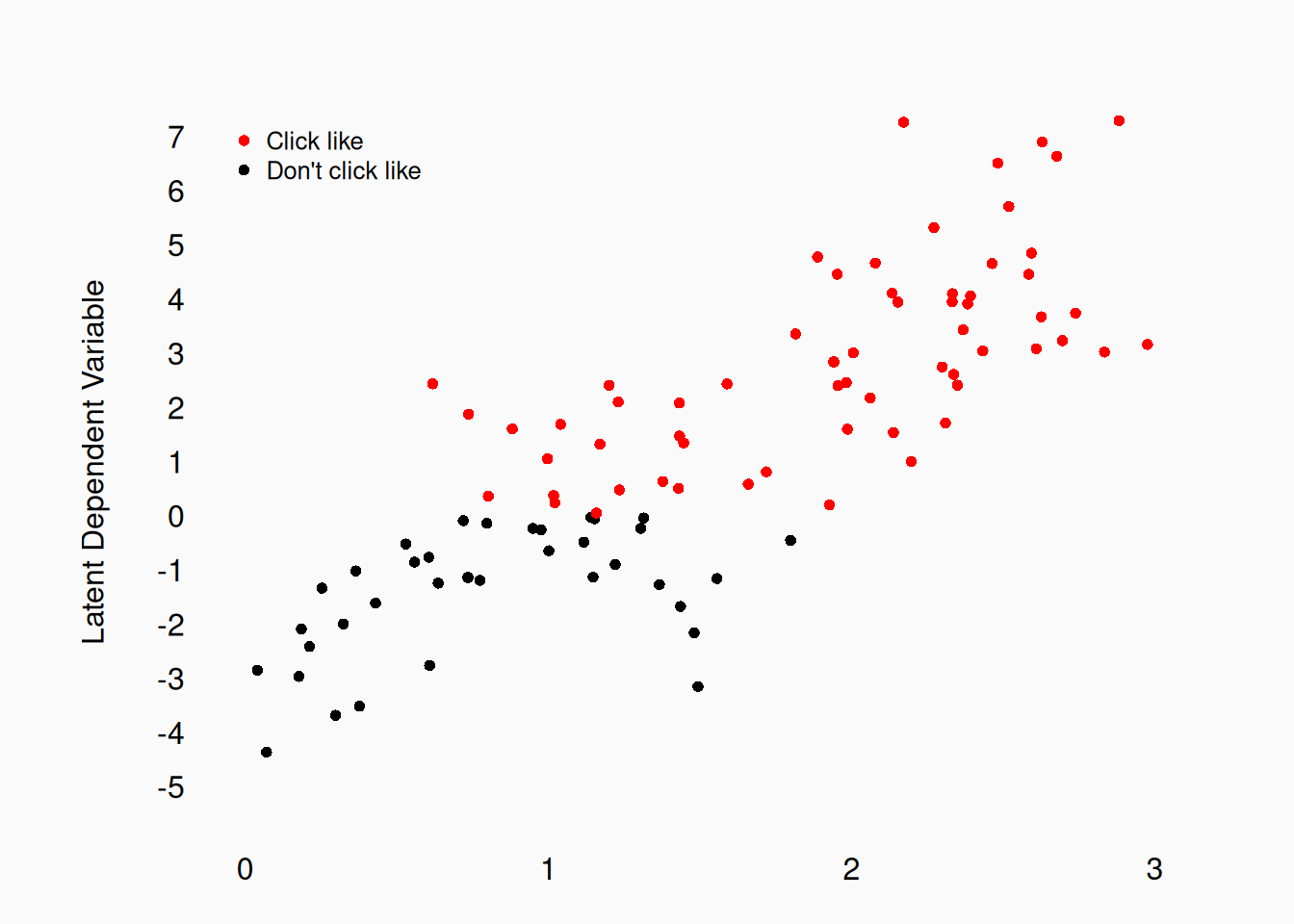
The latent linear variable \(z\) is converted to probabilities using the “logistic” link function \(\frac{e^{z}}{{e^z} + 1} = p\), and \(\epsilon \sim \mathcal{Binom}(1, p)\). (The shape of the logistic curve looks similar to the probit curve, but is a little different.)
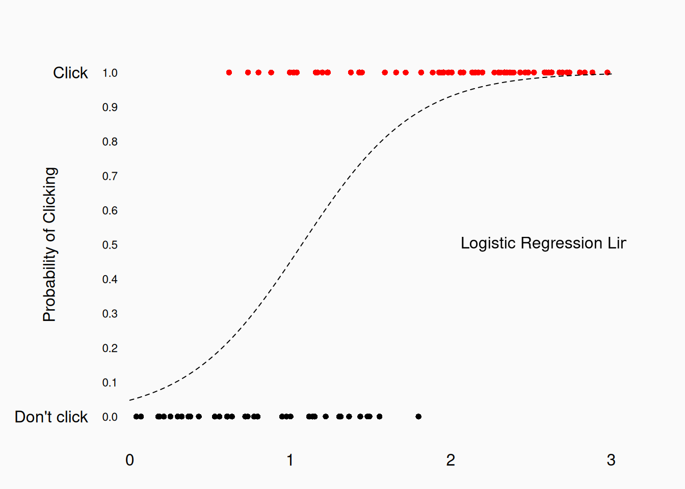
Logistic regression is the most fundamental binary classification model in both statistics and machine learning. The logistic (or probit) error model can be extended to any type or combination of independent variables (main effects, interactions, etc.). So, for example, in addition to logistic regression, you can also do “logistic t-tests” or a “logistic ANOVAs.”
If the normal distribution is so important and common, why not use the probit model instead? Why do we favor logistic regression over probit? One reason is that the latent logistic variable is (slightly) easier to interpret: It’s the log odds. In other words, in logistic regression, the latent variable represents the log of the odds \(\log(odds)\). So if the latent variable has a value of \(.7\), that means the odds of click (for example) would be \(e^.7 = 2.013\)—about two to one. This means that \(p = \frac{2.01}{2.01 + 1} = .668\). This is the link function that creates the logistic curve.
Let’s look at our logistic regression example:
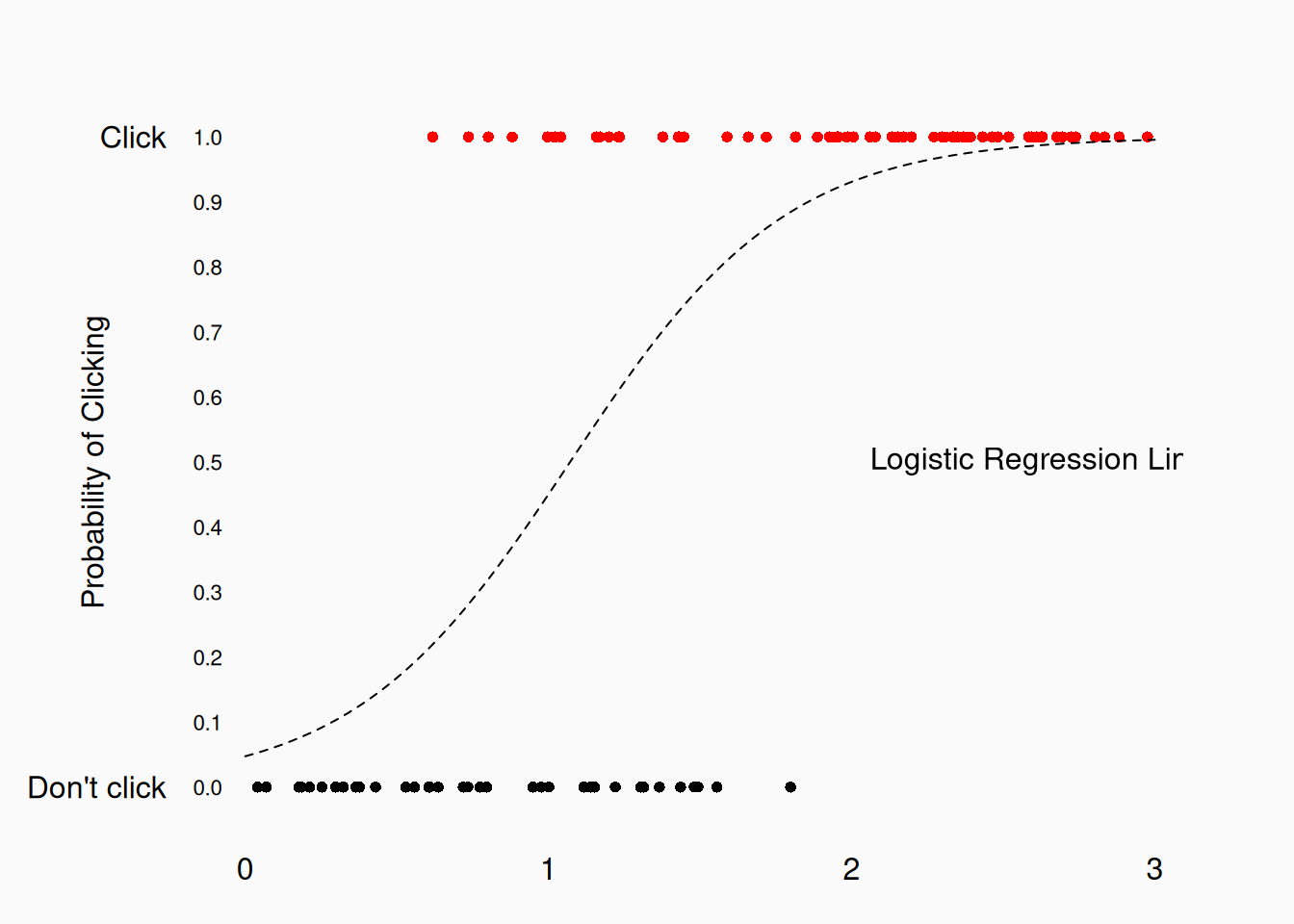
The slope of the latent variable is \(2.8\); \(e^{2.8} = 16.4\). This means that “Every one-unit increase in the independent variable makes the odds of clicking ‘Like’ multiply by 16.4.”
Ordinal Categories
What if our dependent variable is more than two (ordered categories)?


We’d need an ordinal regression. We can easily extend the conceptual model we are using: perhaps a linear latent variable is being binned into three categories.
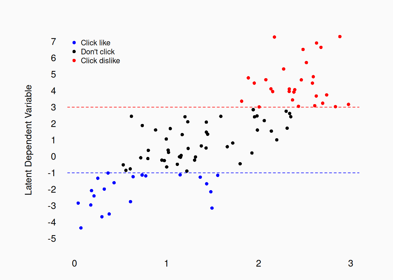
This can work well. However, the result depends a lot on what those cut offs are (I chose 3 and -1). In practice, those ordinal cutoffs become more parameters that we have to estimate in our model, so it’s a bit more complex than logistic/probit regression.
Complex models
Another approach to dependent Variables which are ordinal, or unordered, categories is to model the data using \((k - 1)\) logistic regressions. In other words, we might postulate that there are two latent variables:
- a “how strong is my opinion?” variable, which determines whether a user bothers clicking at all, and
- a “what is my opinion?” variable, which determines which button they click (if they click at all).
We could model this with one logistic regression predicting if a user clicks at all and a second regression predicting which button they click. These sorts of models can be estimated by searching for the maximum likelihood solution.
A multiple-logistic-regression approach can also be applied to ordinal data. Perhaps you have four ordinal categories \(\{A, B, C, D\}\). We could construct three logistic regressions that are chained together:
- Predict \(A\) vs \(\{B, C, D\}\)
- Predict \(B\) vs \(\{C, D\}\)
- Predict \(C\) vs \(\{D\}\)
We can also use this approach for arbitrary (unordered) categories. If you have \(k\) categories, you can always break them up into a hierarchy (you must choose) of \(\log_{2}(k)\) pairs. The parameters you get will depend on what pairings (hierarchy) you choose, but the model fit should turn out (more or less) the same no matter how you do it.
Mixture Models
In the previous example, I showed how we can model one set of data with multiple (simultaneous) logistic regression models. In fact, there are many other ways we can use multiple linear models to model complex dependent variables. Consider this data:
numeric(0)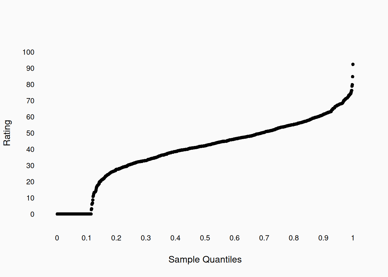
About 10 percent of the time, the measurement is zero, but the rest of the time the measurement is normally distributed. We could use a logistic regression model to predict whether the rating is zero and a separate linear model for the non-zero observations. This is an example of a zero-inflated model.
Once we start piecing together complex models like these, there are many possibilities. When constructing complex models, we should always consider two questions:
- Is this a valid mathematical model of the data?
- Is this a valid conceptual model of the data?
We need to answer these questions for ourselves, but we will also need to convince our audience and reviewers. Ideally, we should design models a priori to limit the chance of overfitting and Type 1 errors.
What does “robust” mean in statistics? It means that even if the assumption is wrong—in this case, that the error isn’t really exactly normal—the Type-1 error rate isn’t affected much. (Classical statistics is all about that Type-1 error rate!)↩︎
Our operational definition of “liking,” enforced by our measurement protocol, is binary.↩︎