57 Pitfalls of NHST

(Modified on 2026-08-11)
3,465 words

The Null Hypothesis Significance Test (NHST) procedure is designed to control the rate at which we make false research claims (Type 1 errors). Unfortunately, it is surprisingly easy to thwart this goal. The NHST is very sensitive to the exact procedure we employ and this can lead to subtle, unintuitive errors.

Subtle details of our analysis protocols can affect our results.

The problems discussed in this chapter are well known and widely discussed in the context of null hypothesis significance tests. However, these problems generalize to all research, even if we rely on alternative approaches to hypothesis testing (i.e., cross-validation or Bayesian statistics). Thus, the lesson presented in this chapter—namely, that even subtle details of our analysis protocols can affect our results—is relevant to all researchers. However, NHST makes some of these problems especially obvious, and we can use NHST as a case study to investigate and explain exactly how and why they happen. In other testing paradigms, the problems may still be there, but may be less obvious.

In the Spring of 2024, I worked with my students Venkat Krishnan, Noel Alben, and Anish Nair (they did most of the work) to create a new dataset of Carnatic music performances, Sanidha. Sanidha is the first such dataset to feature isolated audio tracks for each instrument (including the vocals), making it ideal for source separation research.

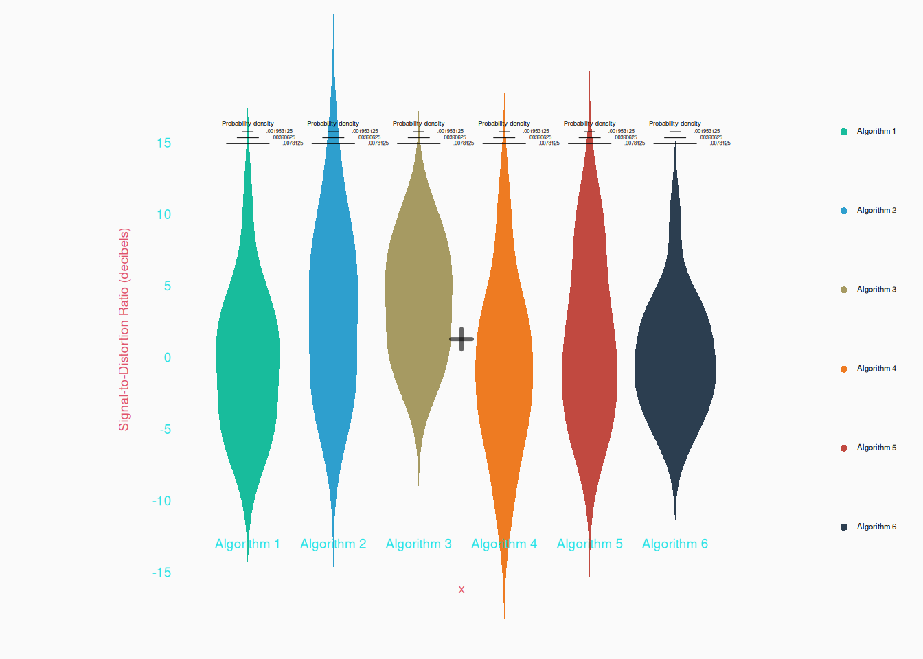
To test Sanidha, we might consider testing the performance of five different vocal separation algorithms on the data. If we apply each algorithm to all the isolated passages in Sanidha, and calculate the signal-to-noise-ratio (SNR) between the algorithm output and the true isolated stem, we end up with data that looks like this:

It appears that Algorithm 3 works better than the others. But we are skeptical scientists right? So we should run a statistical test, comparing the performance of algorithm 3 to the other algorithms. If we run this is as a \(t\)-test we get the result: \(t(88)=2.287\), \(p < .05\)—a significant result!

There is a problem with this. The statistical test I’ve run here isn’t actually reflective of the actual procedure I used. Why? Because we actually slipped an extra step into our procedure: we first looked at the data and picked out the algorithm with the highest average score; we then compared this algorithm to the rest. Why is this a problem? Well, even if the null hypothesis was true, every time we sampled data one of the algorithms would always happen to do better than others, by chance. By picking out that best algorithm post hoc we are actually biasing the test.

We can show this bias by actually simulating our whole procedure, with the null hypothesis being true in all our simulations. These will be the steps in our simulation:

Randomly sample data from a single distribution (since we are simulating the null hypothesis is true, all samples come from one distribution).
Calculate the means of the (random) data within each group (algorithm).
Pick the algorithm which has the highest mean.
Compute a \(t\)-test, comparing the highest-performing algorithm to the other algorithms, and get the \(p\)-value.

Here’s the code:

n <- 600
algorithms <- gl(6, 100, 600, labels = paste0('Algorithm ', 1:6))



pvalues <- sapply(1:10000, \(i) {
  SDR <- rnorm(n, 2, 5) # random sdr values
  means <- tapply(SDR, algorithms, mean) # means of each group
  
  best <- names(which.max(means)) # name of best algorithm
  
  bestvsrest <- algorithms == best
  
  t.test(SDR ~ bestvsrest)$p.value
})

And the result? Let’s plot those 10,000 p-values, sorted from lowest to highest. If everything is working correctly, only 5% of p-values should be under .05. But what do we see?:

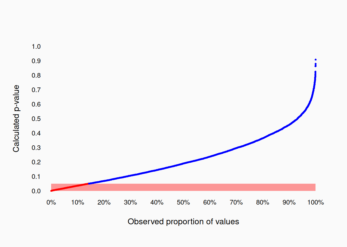
In this case, the \(p\)-value we calculated was lower than .05 about 15% of the time: that’s not supposed to happen! Since the null hypothesis in the simulation is true, the \(p\)-value should only be less than \(.05\) 5% of the time, not 15%! Statisticians describe this as an example of an “inflated” Type-1 error rate.

The fundamental problem here is that we are basing our statistical procedure on a post hoc judgement. We only decided to test Algorithm 3 after we looked at the data. The trick is that we can’t just consider what we did, but what we would have done if the data looked different. If the data had looked differently, we would have picked a different algorithm to test. In contrast, if we a priori decided to test Algorithm 3 only, always, then our Type-1 error rate would be the correct \(.05\).

Stopping Condition

Consider another example. Let’s say that you are conducting a behavioral experiment to test the hypothesis that there is a negative linear relationship between personality and the ability to identify musical intervals. You design an experiment where human participants listen to and attempt to identify forty intervals and then take a personality questionnaire. You manage to recruit seven participants, giving you 280 data points in total. You conduct a null hypothesis significance test on your data, but the result is not significant. However, a graph of the data does look more-or-less like you predicted—there looks like there is an effect, but the test is not significant because there is too much noise. It seems plausible¹ that you could be making a Type-2 error, simply because you don’t have enough data—seven participants is really small for a music-cognition experiment, after all. So you gather some more data, until you have twenty participants in total. Unfortunately, the test is still not significant. However, you know that most behavioral psych researchers aim to recruit more like 40–50 participants, so you decide to keep going. Once you have 45 participants, you conduct your test again, and now the result is significant (\(p < .05\)). Awesome! You can publish your positive finding! What could be the problem?

The problem is that you used post hoc information to decide when to stop collecting your data: this is called your “stopping condition.” Let’s simulate this scenario and see what happens: remember, we have to simulate the whole procedure, including what we would have done if the data was different. Our procedure went like this:

Gather seven participants and conduct a NHST.

If the test is significant, stop gathering data and publish!
If the test is not significant, keep going.

Gather thirteen more participants and conduct a NHST.

If the test is significant, stop gathering data and publish!
If the test is not significant, keep going.

Gather 25 more participants and conduct a NHST.

If the test is significant, stop gathering data and publish!
If the test is not significant, keep going.

How long would we keep going? Until we run out of time or funding?

Let’s assume that after 45 participants we would stop no matter what…but would we?

I will now simulate the scenario above, where the null hypothesis is true, and see how many Type 1 errors we make:

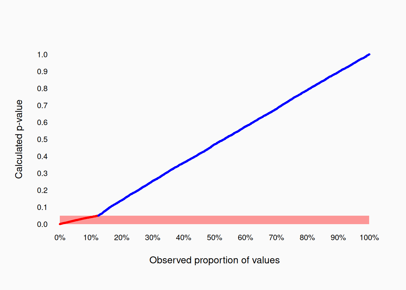
Our Type 1 error rate is well over 10%. The key thing is that we would have stopped earlier if we saw a significant effect earlier. If we always planned to gather 45 participants report the result, then there would be no problem.

The problem we are grappling with here can be unintuitive, so let’s try explaining it one more time. In this scenario, we conducted three different significance tests, with \(N\) equals 7, 20, and 45 respectively. If we look at the \(p\) values of these three tests we see something like this:

\(N = 7 \implies .05 < p\)
\(N = 20 \implies .05 < p\)
\(N = 45 \implies p < .05\)

Two are non-significant, one is significant, but we go with the significant test. Imagine, if instead we had seen this:

\(N = 7 \implies .05 < p\)
\(N = 20 \implies p < .05\)
\(N = 45 \implies .05 < p\)

Again, one of our three tests is significant, but would you want to take this \(N = 20\) and publish it as a positive result? This is obviously questionable—but in reality, if the \(N = 20\) test had been significant, we wouldn’t have bothered with testing \(N = 45\) at all, and would have happily gone with the significant test from \(N = 20\). If we had these three tests, the only appropriate thing would be to report the \(N = 45\) test, regardless of the outcome. We can’t choose which test to report based on the outcome of the test!

Multiple Comparisons

The greatest challenge to hypothesis testing, in NHST or otherwise, is the problem of multiple comparisons—also known as “multiple tests.”

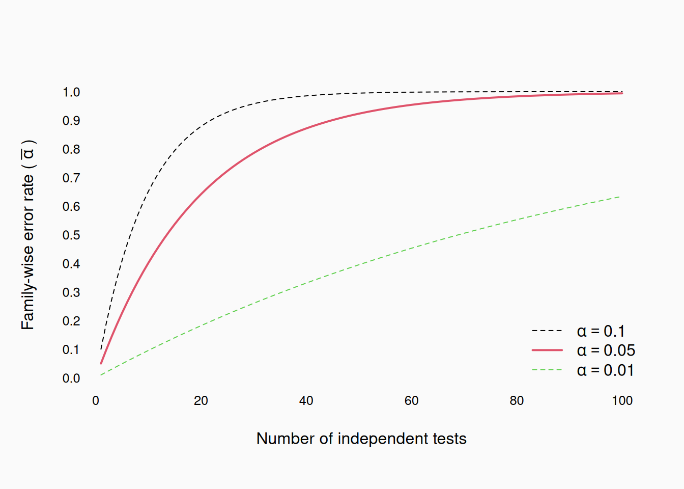
Whenever we conduct a test, there is a chance that the outcome of the test is a mistake. For example, in the case of NHST, we make sure that the chance of making a Type-1 error is at most \(.05\). But, what if we conduct more than one test? Well, if we assume the tests are independent (and the null hypotheses are both true), then the chance that both tests would result in a Type 1 error would be \(.05^2 = 0.0025\). However, the probability that at least one test would be significant would be \(1 - (1 - .05)^2) = 0.0975\). By the same logic, if there were five tests conducted, at least one would be significant \(1 - (1 - .05)^5 = 0.2262\). This “chance of at least one error” is called the family-wise error rate, usually represented as \(\bar{\alpha}\). Generally, \(\bar{\alpha} = 1 - (1 - \alpha)^n\), where \(n\) is the number of independent tests. As the number of tests increases, the family-wise Type-1 error rate grows rapidly:

Suppose you are browsing through a recent issue of a scholarly journal. The issue contains twenty empirical research articles. Each article reports positive results in testing a single hypothesis (using \(\alpha = .05\)). By the logic above, there’s a 64% chance that at least one of the papers has published a spurious result (a Type-1 error).

Now suppose you were reading a single published article. The article reports statistical tests for twenty hypotheses: the researcher reports that three of the hypotheses are statistically significant (\(p < .05\)). In this case, we’d actually expect to see three (or more) falsely-significant tests more than 7% of the time!

Now suppose that I run an experiment, whose results turn out to be negative (\(p > .05\)). I know that negative results might arise for all sorts of reasons. Perhaps the reason why it didn’t work is because of poor equipment calibration. I carefully re-calibrate the machine and repeat the experiment. Still, it doesn’t work. The participants report that they find my experiment very boring, and I begin to suspect that my data are less than ideal because the participants are not fully motivated. I decide to cut the number of stimuli in half and compensate for the loss of data by doubling the number of participants. Once again, I re-run the experiment, and once again I end up with negative results. At this point I am suspicious about the quality of my participants. I would like to use better musicians, so I administer a pre-selection test that allows me to gather data from the subjects who are the most musical. Once again the results turn out to be negative.

With much hard work over several months, I continue to refine my experiment, removing sources of error, aiming for greater reliability in responses, and so on. Finally, after the 20th attempt, I get positive results (\(p < .05\)). Hurray; My hard work has finally paid off!

Of course, repeating any experiment twenty times means that, even if the null hypothesis was true, I’d expect to see a (falsely) significant result 64% of the time! My efforts to “improve” the quality of my experiment may, or may not, have done anything. But just by running the experiment multiple times I increased the likelihood of producing a spurious positive result.

What these examples illustrate is that multiple comparisons happen all the time. They happen when we test multiple hypotheses. They can also happen when we run several versions of an experiment, or by “tinkering” with various criteria when analyzing your data—for example, excluding outlier data (or not), or changing our stopping condition.

Dependent tests

If we are considering two tests reported in two separate papers, conducted by two different groups of researchers, it makes sense to consider the tests statistically independent. This makes it easy to calculate the family-wise error rate, as I did above. However, when conducting multiple tests using the same dataset, or using the same procedure, it is likely that the tests won’t be entirely independent. In other words, if we are testing two hypotheses using a particular set of data or methodology, the results are correlated: meaning, that if one test is significant, the other test is somewhat more likely to be significant too (or vice versa). The obvious extreme is that if you run the same test twice on the same data the tests are 100% correlated, and the family-wise error rate is the same as the singular \(\alpha\) level (\(.05\)).

In situations where tests are dependent, the true family-wise type-1 error rate won’t climb as high as the graph shown in the previous section. How fast will it grow? It’s hard to say: it depends on how dependent the tests are, and there’s no general approach to calculating what the family-wise error rate will be.

Accounting for Multiple Tests

There are a few ways we can try to account for the problem of multiple tests. The most basic way is to limit the number of tests you perform. Resist the temptation to test many hypotheses, especially if they are related hypotheses. Instead, focus on testing your important hypotheses, ideally those which you identified a priori.

Unfortunately, in some cases, we can’t avoid doing multiple tests—we simply have multiple hypotheses to test. In these cases, we must “correct for” multiple comparisons in our statistics. This is done either by: 1) “correcting” our \(p\)-values or 2) “correcting” our \(\alpha\) level. These two approaches are actually equivalent: for example, we could either double all our \(p\)-values or divide our \(\alpha\) level by two—the result is the same either way.

Independent tests

The most basic multiple-test correction is called the Bonferroni correction: simply divide \(\alpha\) by the number of tests.² Notice, that this approach is overly conservative, meaning that it over-corrects for the problem. A better approach is to use the formula from above (\(1 - (1 - \alpha)^n\)) to correct our \(\alpha\), so we get the exact right numbers for \(n\) independent tests. This is called the Šidák correction. Unfortunately, even the Šidák correction is overly conservative when our tests are correlated, which will generally be the case. By using tests that are overly conservative, we are over-correcting for type-1 errors, and thus inflating our type-2 error rate, which is not ideal.

Dependent tests

Fortunately, there are ways of correcting for multiple comparisons while considering the correlation (dependence) between tests. This means we can avoid being overly conservative (and thus needlessly inflating our type-2 error rate). Unfortunately, as I mentioned above, there is no general way to do this, because it depends on how the tests are correlated. Instead, there are specific methods designed for specific statistical tests.

The most common specialized corrections are used in the context of the Analysis of Variance (ANOVA). The basic ANOVA test is used to test the “omnibus” null hypothesis that a set of three or more sample means are all the same. For example, returning to the source-separation data evaluation example from above:

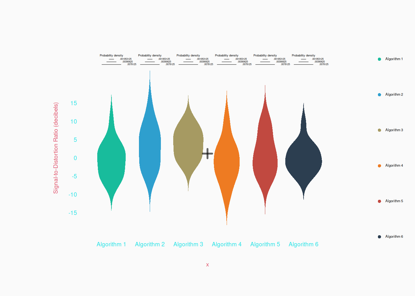
An ANOVA would test the null hypotheses that these six samples are actually sampled from a single population. In this case, \(F = 2.37(\frac{5}{84})\), \(R^2 = .12\), \(p < .05\), so the null hypothesis doesn’t seem to be consistent with the data. But, returning to the start of the chapter, what if we wanted to know if Algorithm 2 is better than Algorithm 4, or whether Algorithm 1 is better than Algorithm 6? Now, ideally we should have decided which comparison tests we wanted to conduct a priori and just conduct those. But very often, we will want to conduct some post hoc pair-wise comparisons—in fact, we might want to compute all of them (all fifteen pairs of groups). We could use the Šidák correction and set \(\bar{\alpha} = 0.537\); however, this is overly conservative because it assumes the tests are independent. Instead, we could use (for example) Tukey’s range test, which corrects for multiple post-hoc comparisons of levels in an ANOVA, while maximizing statistical power (minimizing type-2 errors).

Invisible Multiple Tests

Multiple tests are not always immediately apparent. Sometimes we need to be vigilant to recognize situations where multiple tests are occurring.

In the first example from this chapter, we tested whether the best algorithm, Algorithm 3, really works better than the others, and why this is problematic. Another way of thinking of this is that we implicitly did multiple comparisons: we compared all of the different groups (by eye) and picked the test that was most likely to be significant. If we had, for example, used a conservative correction and used \(\bar{\alpha} = \frac{.05}{6}\), our test would have not turned out significant in the first place.

One of the most insidious problems facing the scientific community, is a problem of invisible multiple tests at a community-wide scale.

Research reporting positive results is 2–3 times more likely to get published than research reporting negative results. Moreover, research indicates that researchers are less likely to submit negative reports for publication. This phenomenon is referred to as positive results bias.

Suppose that there is a popular theory—let’s call it Theory A. Researchers in the field think Theory A has a lot of merit: it is conceptually beautiful and makes intuitive sense. A young scholar named Alice is interested in Theory A; She does a literature search and is surprised to find that no experiment has been published testing Theory A. Alice decides to carry out a pertinent experiment. She designs and carries out an experiment, but is disappointed when she gets negative results. She wonders about her design. There are a number of improvements that she might make, but she is discouraged from continuing. Alice abandons the project, takes her data and places it in the bottom drawer of her desk.

Another scholar, Bill, has been thinking about Theory A. Bill’s dissertation research had assumed that Theory A was true and he’s always been a little uneasy about this assumption. Everyone thinks Theory A is uncontroversial, but Bill’s literature search fails to find any experiment testing Theory A. Bill decides to carry out an experiment with the hope that he can find evidence consistent with Theory A. He designs and carries out an experiment, but is disappointed when he gets negative results. He submits a manuscript to a professional journal, but the reviewers are skeptical. Theory A is conceptually beautiful and makes intuitive sense. There are several ways in which Bill’s experimental method could be improved. The editor of the journal requests a “revise and resubmit.” Bill makes some changes to his method and runs the experiment again. Still, he gets negative results. He knows the journal reviewers will be unhappy that he didn’t implement all of the (sometimes impractical) changes they suggested. Discouraged, he places his manuscript in the bottom drawer of his desk and goes on to other projects.

Alice and Bill are not alone. Over the years, several other scholars attempt to test Theory A without success. There is a good reason why all of these experiments end in failure: Theory A is, in fact, wrong. All of the negative results are telling us something, but because of a positive results bias, the results are hidden from view. This is the bottom drawer effect.³

While the bottom drawer effect is pernicious, the situation can sometimes get even worse. Consider how the story might continue…

Many years later, Zack decides to test Theory A. Zack is not aware of the many other tests that have been done that all ended in failure. Zack carries out an experiment and is thrilled to get positive results at the .05 significance level. Zack immediately submits the results to a prestigious journal. The journal reviewers are delighted to see a study that “confirms” a widely loved Theory A, and the journal Editor is thrilled to publish an article that will surely become frequently cited. There is only one problem. In reality, Theory A is wrong, and Zack has had the misfortune of getting spurious results. Repeat an experiment enough times, and one is bound to get spurious statistically significant results. Dozens of previous experiments resulted in negative results. Zack’s experiment is really part of a pattern of multiple testing: the p value in Zack’s experiment ought to be corrected for the many earlier tests. But Zack (and everyone else) is unaware of all of the other tests that have been carried out by other researchers. The bottom drawer effect has become a version of the multiple tests problem—one that is aggravated by positive results bias.

Sometimes multiple tests are not recognized by a researcher. Suppose, for example, you have a set of sound stimuli in which you are interested in the effect of a certain manipulation on perceived emotional content. You ask listeners to judge a number of different affective states: happy, ecstatic, sad, grief, tender, aggressive, dramatic, relaxing, inspiring, contemplative, etc. If you test each affect separately, then you will have to correct for multiple tests.

Inexperienced researchers will sometimes go on a “fishing expedition” in which they test many different hypotheses against the data they have collected. For example, the researcher may test 30 or 40 hypotheses. However, only two or three hypotheses produce significant results. They then craft a paper “testing” these three hypotheses without ever mentioning that they tested a large number of other hypotheses. We might call these unreported tests.

Incidentally, it is okay to engage in such “fishing expeditions” if your research inquiry is exploratory, not hypothesis-driven. For example, you might carry out 30 tests on a set of data, and find two (seemingly) statistically significant results. Given the number of tests carried out, there is a good chance that either one or both of these results are spurious. However, you might be sufficiently intrigued to carry out a separate study whose purpose is explicitly to test one or both of these hypotheses. In other words, we can “mine” a data set for new ideas, that are then independently tested (i.e., explore-then-test).

Mantras

This chapter deserves its own dedicated mantra:

With many tests comes great responsibility

Multiple at bats gives you multiple chances to get lucky. It’s not a test if you retake it until you get an A. If you give yourself enough chances, you’ll eventually hit a home run.

Each statistical test increases the likelihood of making a Type-1 (false positive) error. Repeating an experiment also increases the probability of a Type-1 error.

In fact, it is plausible.↩︎
Alternatively, multiply your \(p\)-values by the number of tests.↩︎
For musical examples of the bottom drawer effect, see Mashinter (2006).↩︎