54 Factor Analysis
(Modified on 2026-08-12)
2,215 words
Factor analysis is a statistical method that can be used to reduce or distill many variables into a smaller number of variables (called factors). Many variables are highly correlated, and this suggests that there is an underlying cause responsible for the similar behavior of correlated variables. This unobserved variable can be regarded as “latent” in the data. The purpose of factor analysis is to expose or reveal possible latent variables.
An example of the use of factor analysis is found in a study by Thomas Schäfer and Peter Sedlmeier (2009). They asked 507 Germans to rate how well they liked 25 musical styles. Of course people have different preferences: Some people like classical music, some like jazz, and some like rock. But it is not simply the case that people like one style and are indifferent to other styles. For example, a person might most prefer jazz, but also enjoy reggae. It turns out that there are broad patterns evident in people’s likes and dislikes. For example, a person who likes goth is also likely to enjoy punk and metal. People who like gospel also tend to enjoy soul. People who like folk music are more likely than other people to enjoy country music. Factor analysis uses the correlations between different variables to reduce the number of independently varying qualities.
In their factor analysis of stylistic preferences, Schäfer and Sedlmeier found an underlying commonality between techno, trance, dance and house. Whatever it is that causes a person to like any one of these also tends to dispose that person to like the others as well. In other words, factor analysis suggests a common cause that leads to a preference for all four styles.
The table below identifies the so-called factor “loadings” for 25 musical styles on the six dimensions arising from the factor analysis carried out by Schäfer and Sedlmeier.
| Style | Sophisticated | Electronic | Rock | Rap | Pop | Beat, folk, & country |
|---|---|---|---|---|---|---|
| Jazz | .81 | |||||
| Blues | .77 | |||||
| Swing | .70 | |||||
| Classical | .69 | |||||
| Techno | .88 | |||||
| Trance | .87 | |||||
| House | .77 | |||||
| Dance | .71 | |||||
| Punk | .77 | |||||
| Metal | .70 | |||||
| Rock | .67 | |||||
| Alternative | .66 | |||||
| Gothic | .56 | |||||
| Ska | .54 | |||||
| Hip hop | .73 | |||||
| Rap | .71 | |||||
| Reggae | .66 | |||||
| Pop | .82 | |||||
| Soul | .64 | |||||
| Rhythm & Blues | .63 | |||||
| Gospel | .55 | |||||
| Beat music | .69 | |||||
| Folk | .67 | |||||
| Country | .67 | |||||
| Rock & roll | (.46) |
Notice that the factor analysis points to an underlying commonality between jazz, blues, swing and classical. It is important to understand that these styles are not a “cluster.” They are simply the variables that exhibit the greatest “loading” on the proposed factor. Other likes & dislikes may contribute to this factor, but these four contribute the most. It’s also important to note that not everyone will share the same constellation of tastes. For example, not everyone who enjoys jazz will enjoy classical, and vice versa. Instead, there is an underlying “something” that seems to encourage people to like jazz, blues, swing and classical, more than other styles. Notice that jazz (.81) and blues (.77) load on this factor more than swing (.70) and classical (.66).
Instead of referring to a factor as “Factor 1” or “Factor 2,” it is often helpful to refer to a factor by giving it a name. For example, Schäfer and Sedlmeier, decided to refer to the first factor using the name “sophisticated.” Similarly, they decided to refer to the second factor (with high loadings on techno/trance/dance/house) using the term “electronic.” It is important to understand that these names are interpretations offered by the researcher, and that there is no official status to these labels. Other researchers may disagree with a factor name, and in some cases the name may be deceptive or reflect researcher bias. For example, one could argue that the jazz/blues/swing/classical factor might be better labelled “born before 1960,” while the punk/metal/rock/alternative/gothic/ska factor might be better labelled “born between 1965 and 1980.” Factor analysis does not tell you the source or reason for the underlying factor; it simply indicates that such a factor probably exists.
It is important to understand that factor analysis doesn’t simply discard some of the original variables. In Schäfer and Sedlmeier’s (2009) analysis of styles, the factor analysis is not merely a way to reduce the number of styles. The styles may be truly distinct, and one style can’t simply be regarded as a “variant” of some other style. Instead, the underlying factors may relate to entirely different phenomena. For example, the factors accounting for stylistic preferences might relate to age, race, geography, or parental educational attainment. Factor analysis doesn’t mean that soul and rhythm & blues are similar. It means that whatever causes a person to like soul is similar to whatever causes a person to like rhythm & blues. Similarly, a liking for jazz shares some underlying cause with a liking for classical music — even though the styles are clearly different.
Factor analysis is similar to another statistical method known as Principal Components Analysis (PCA). The two methods use different numerical methods, but share many commonalities. An important difference between PCA and factor analysis is that factor analysis can also be used to test an a priori theory. Suppose, for example, that you have a theory that there are four factors contributing to the quality of a musical performance. Factor analysis can be used to test your theory, determining the probability that the observational data are consistent with the four proposed factors. So in addition to providing a method for exploratory data analysis, factor analysis can also be used as an inferential test — a way of testing a prior hypothesis.
Multi-Dimensional Scaling
In simple terms, multi-dimensional scaling amounts to creating a map from a list of distances.
Suppose we have a list of the distances between major American cities. The distance between New York and Chicago is 714 miles. Between New York and Los Angeles it is 2,462 miles. Between Chicago and Los Angeles it is 1,744 miles. And so on. A computer program can be used to construct a map, simply using the distances. For example, the program begins by arbitrarily placing one of the cities (say New York) on a blank page. With New York in the center, it then draws a circle with a radius of 714 miles; Chicago lies somewhere on this circle. Similarly, it draws another circle with a radius of 2,462 miles; Los Angeles lies somewhere on this circle. It then chooses a point on the first (Chicago) circle, so that it is 1,744 miles from a point on the second (Los Angeles) circle. It continues in this way until all of the cities have been plotted.
The first thing to notice about this map is that the orientation of the map is undefined. The map could be drawn with “North” in any direction. Moreover, it could also draw the map inside-out. We are used to viewing maps from the “above” perspective — as though the viewer is floating in the sky. However, our resulting map might have been produced as though the viewer were positioned below ground looking up.
The second thing to notice about the map is that it will require a slight amount of “stretching.” The distance measures are not exact, so the point representing a given city might be pushed and pulled a little bit. Technically, the amount of stretching is referred to as stress. Each multi-dimensional scaling solution (each map) will be accompanied by a numerical value representing the total stress.
If the stress becomes too great, the MDS solution will add an additional dimension. Suppose for example, that our map included major cities of the world, not just American cities. You cannot draw a map of the world in two-dimensions while preserving accurate distances. The MDS solution will “pop” into three dimensions, and we will soon see that the positions of the various world cities are best represented using a three-dimensional sphere.
What’s important is that MDS constructs these “maps” from lists of paired distances. MDS is quite robust — so that the distances don’t have to be exact. Suppose, for example, that we asked you to estimate all of the distances between various major cities. What is the distance between New York and Chicago. Perhaps you guess 500 miles (instead of 714). What is the distance between New York and Los Angeles. Perhaps you guess 2,000 miles. (instead of 2,462). And so on. Based solely on these distance estimates, MDS will manage to create a remarkably convincing map. Once again, it will do some “stretching” to make things fit. But the map from estimated distances will typically be very close to the map for the real distances — although the “stress” value will be higher.
Now suppose we use this technique, not to represent physical distances, but psychological distances. By way of example, John Grey (1977) played pairs of tones to listeners (e.g., clarinet and flute, clarinet and trumpet, clarinet and violin, etc.), and asked participants to judge the similarity of the tones on a numerical scale. Using this approach, the average distance between clarinet and flute might be 3.6, whereas the distance between clarinet and xylophone might be 9.1. With enough paired comparisons, Grey could use MDS to portray the sounds in a multi-dimensional space, where similar timbres are close to each other.
Grey’s tones were mapped in a three-dimensional space. MDS does not “label” the dimensions. That interpretation is left to the researcher. By traversing through the tones along a single dimension, one can hear what changes along that dimension. In this way, Grey was able to interpret one of the dimensions as “brightness.” Sounds at one end tended to be darker, and they got brighter as one moved along the dimension. Grey was able to interpret another dimension as the percussiveness of the sound, and so on. In short, MDS allows the researcher to glimpse the underlying factors used by listeners when judging the similarity of the tones.
In general, multi-dimensional scaling starts with a matrix of item-item similarities, and then plots the items in some space so as to preserve the similarity relationships. MDS is an exploratory data analysis method that allows the researcher to view items of interest in some sort of spatial representation where distances are meaningful.
Pitch
Suppose we played many pairs of pitches and asked people to judge “the similarity” between the pitches. We might provide a scale of 1 to 10, where 1 is very close, and 10 is very distant. A listener might judge the pitches D4 and D#4 to be “quite similar” and give them a value of “2.” Conversely, the pitches C2 and F#6 might be deemed very different, and be given a value of “9.”
Of course, pitches can be “similar” in other ways. For example, listeners might judge the pitches E3 and E4 to sound “quite similar.” As a result, the similarity ratings between E3 and E4 might be quite close — say “1.”
This state of affairs might lead to a seemingly odd arrangement. On the one hand E4 might be very similar to D#4; E4 might also be very similar to E5; however, D#4 might be heard as rather dissimilar to E5. Despite this apparent paradox, multi-dimensional scaling will have no difficulty dealing with the situation.
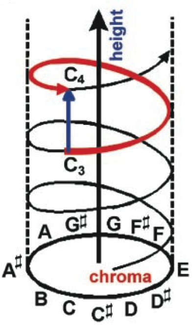
The figure below arises from the MDS solution based on judgments of pitch similarity. Notice that the MDS solution is three dimensional. Two dimensions (circular) relate to what musicians would call pitch-class — what psychologists refer to as pitch chroma. The third dimension relates to the octave — what psychologists refer to as pitch height. It can be seen that in this solution, the pitch E4 is near both D#4 and E5. That is, the two-dimensional solution captures both of the ways in which pitches can be similar.
Medieval Modes
Huron and Veltman (2006) made use of MDS in their study of medieval modes. They assembled a quota sample of Gregorian chants in the eight classic modes: Dorian, hypodorian, phrygian, hypophrygian, lydian, hypolydian, mixolydian, and hypomixolydian. For each mode, they tallied the distributions of the various pitches. They then measured the similarity of the distributions between all pairs of modes: dorian/hypodorian, dorian/phrygian, etc. These distances were then used in a multidimensional scaling procedure. The resulting modal “map” is shown below.
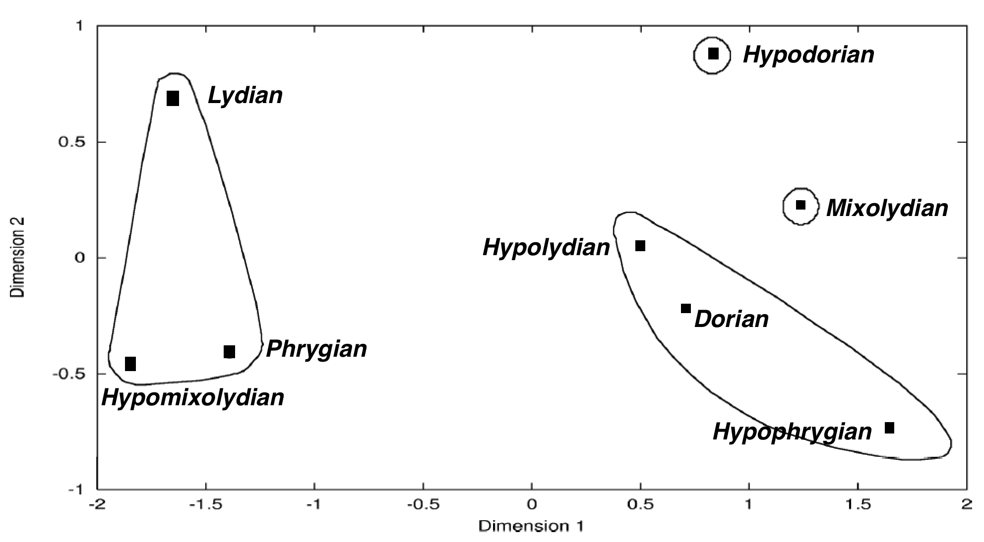
Those modes that are closest together in the MDS solution are the most similar in terms of their pitch distributions. For example, the two modes in the lower left of the graph (hypomixolydian and phrygian) turn out to be statistically indistinguishable.
In the 11th century, a music scholar named Johannes Cotto described the modal system from both theoretical and applied perspectives. Although the theory distinguishes eight separate modes, Cotto suggested that there are only really four modes. These are illustrated in the graph by the circles. Cotto deemed hypdorian and mixolydian as truly separate modes. But the remaining modes group into two practical modes. One group consists of dorian, hypolydian, and hypophrygian. A second group consists of phrygian, lydian, and hypmixolydian. The latter modes all share the pitch C as the tenor tone and appear on the left side of the map. The former modes all share the pitch A as the tenor.
Dimensions 1 and 2 are drawn to scale making it easier to see that Dimension 1 accounts for a greater proportion of the variance. Note the large empty region separating the left and right mode clusters. Dimension 1 suggests a nascent major/minor bifurcation. Although the musical practice represented in the sampled music pre-dates the emergence of major/minor tonality, the results suggest that the possibility for confusion between the modes is already evident in late medieval music, and that the preeminent polarity of confusion is consistent with the later major/minor distinction.