56 Power
(Modified on 2026-08-12)
1,053 words
The main goal of applied statistics is minimizing type-1 errors—false positives. In other words, we want to avoid claiming a hypothesis is true when it is in reality false. This fits our scientific rhetoric: we aim to be skeptical of our own ideas, stack the deck against ourselves, and make many opportunities for our research claims to be falsified.
But what about type-2 errors?—false negatives?
A type-2 error occurs when we claim a hypothesis is false when it is in reality true. Since we focus on self-skepticism and type-1 errors, good researchers actually go out of our way to increase our type-2 error rate. In the context of research, this can mean spending weeks of work designing and conducting an experiment, only to finally conclude that our idea was wrong all along. Now, if our idea is false, then this is obviously the outcome we want.1 However, if our idea is actually valid, and we spend all this time testing it only to falsely reject it (Type-2 error), that’s bad!
There is a long-standing contention in statistics about how much we should worry about Type-2 errors. It would clearly be useful to limit Type-2 errors. However, there is a general fear that if we try to limit Type-2 errors we must inevitably accept more Type-1 error rates and (the argument is) that this is worse. The Type-1-focused approach we use in applied statistics is mainly owed to the ideas of Ronald Fisher. Other famous statisticians like Neyman and Pearson advocated for an approach which considers both types of errors in the 1930s. However, though Neyman and Pearson’s ideas have been influential, in practice, Fisher’s approach has remained dominant to this day.
Statistical Power
The number one goal in applied statistical analysis is controlling type-1 errors (using Null Hypothesis Significance Tests). However, many modern scholars consider consideration of Type-2 error important as well. As we know, we call our Type-1 error rate \(\alpha\); In parallel, we call our Type-2 error rate \(\beta\). However, we will usually talk about \(1 - \beta\), which is called statistical power. Generally, we want \(\beta\) to be small, which means our power is high.
Any decision making procedure must balance Type-1 errors and Type-2 errors. We could always decrease our Type-2 error rate by increasing our Type-1 error rate. For example, if we used \(\alpha = .1\) in our statistical tests, we’d make more Type-1 errors but also fewer Type-2 errors. Conversely, if we try to make even fewer Type-1 errors by setting \(\alpha\) lower—like \(\alpha = .01\)—, we’d end up increasing our Type-2 error rate. The standard \(\alpha = .05\) we use is meant to be a balance between the two types of errors.
To be clear, as skeptical scientists, preventing ourselves from making false claims (type-1 errors) is absolutely our main goal. Thus, we can and do aim to increase our statistical power, but only so long as we can keep \(\alpha =.05\). The reality is that many scholars will appreciate consideration of statistical power, but only if it doesn’t inflate \(\alpha\). If your attempts to increase your statistical power might inflate your \(\alpha\) level, expect to find unhappy reviewers!
Determining Power
Statistical power really depends on three things:
- The \(\alpha\) level, which we aren’t really free to change.
- The effect size we are making a claim about. We don’t ever know what the true effect size is; we only estimate it from our data (or theories).
- The sample size, which is the only factor we have control of! (At least within our resources.)
We can visualize the relationship between effect size, sample size, \(\alpha\), \(\beta\), and power using the sampling distribution of sample means. In the examples below, imagine that we are taking samples of numbers and calculating the sample mean \(\bar{x}\). The null hypothesis is that the population mean is zero. Of course, our sample means will never be exactly zero: If a sample mean is close to zero, our test will be non-significant; if the sample mean is far enough from zero, our test will be significant. Depending on whether the null hypothesis is true or not, we can make correct inferences, or type-1/2 errors. (We will assume a one-tailed test throughout.)
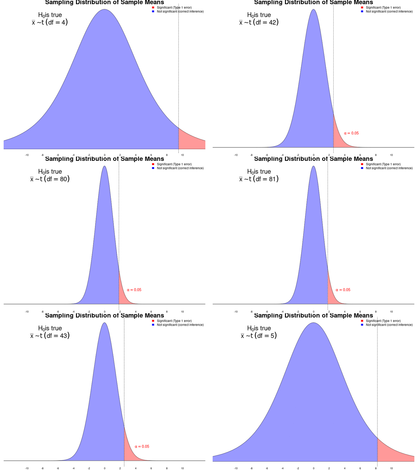
First, consider what the sampling distribution of means will look like when the null hypothesis is true, but we vary our sample size. In this case, we can either make a true inference (non-significant test) or a Type-1 error (significant test):
Notice that, as long as the null hypothesis is true, our type-1 error rate is fixed at \(\alpha\), no matter what the sample size is—this is the whole point of the null hypothesis significance test!
But what if the null hypothesis is false? Let’s see what happens when the true population mean is not zero, but we are still testing the null hypothesis that it is zero. Now, any non-significant test will be a type-2 error:
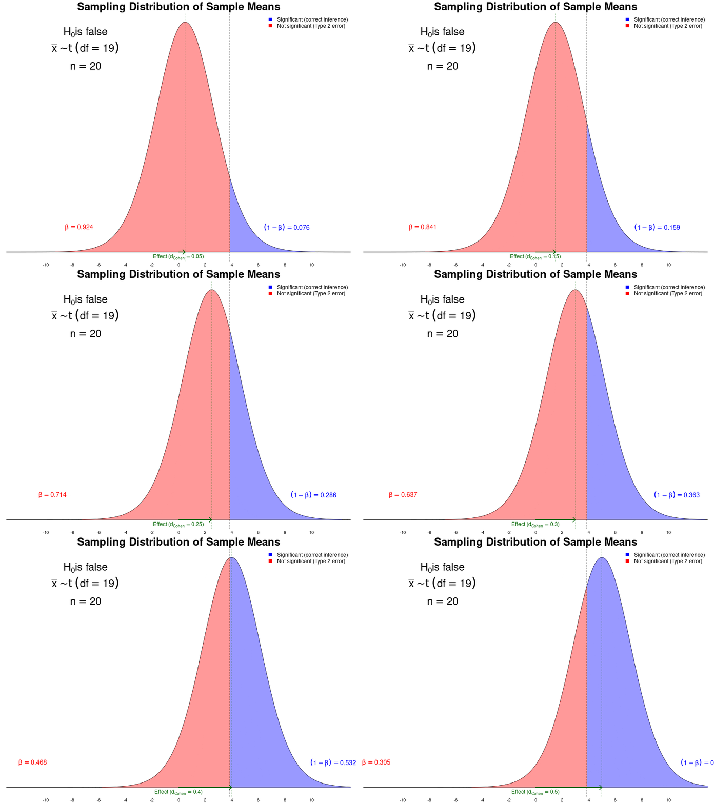
The larger the sample, the less likely we are to make a type-2 error. The stronger the effect, the less likely we are to make a Type-2 error.
Power Analysis
The process of estimating (or planning) statistical power is called power analysis. Power analyses can be conducted a priori, or post hoc.
A priori power analysis is done to estimate how much data you would need to test your hypotheses with a desired power. In order to do this calculation, we have to guess what effect size we will see. The best approach is to consider what would be the minimum effect size that we would actually care about finding, and aim to achieve at least 80% power for that effect (\(\beta = .2\)).
If you are testing how well an after-school music class boosts students’ GPA, perhaps anything less than a \(+0.1\) boost would not be worth bothering with. If the standard deviation of student GPAs is \(\approx.5\), then \(d = \frac{.1}{.5} = .2\) We can then estimate the number of participants we’ll need!
library(pwr)
pwr.t.test(d = .2, power = .8,type = 'one.sample', alternative = 'greater')
     One-sample t test power calculation


              n = 155.9256
              d = 0.2
      sig.level = 0.05
          power = 0.8
    alternative = greater
We’d need 156 independent data points to find this effect 80% of the time. If the effect ends up being stronger, we are even more likely to have a significant test. If the effect is weaker, the probability of us getting a non-significant test—and thus, making a type-2 error—increases, but since we have already established that a smaller effect would be uninteresting anyway, the result could be worse.
When we have a non-significant test, we need to report that our hypothesis failed. However, we might still wonder if we are making a type-2 error. By conducting a post hoc power analysis, we get an idea of how likely it is that we could be making a type-2 error.
Though it might not feel like it.↩︎