50 Null Hypothesis Significance Testing

(Modified on 2026-08-12)
642 words

In the standard (“classical” or “frequentist”) approach to statistics, we use sampling distributions to test our hypotheses. The procedure we use is called Null Hypothesis Significance Testing (NHST).

Science is built on skepticism—especially towards our own work. This is one reason why we will base our statistical tests on the null hypothesis ($H_0$): i.e., that our research hypothesis is wrong. In fact, we assume that the null hypothesis is true. We then specify a statistical model that corresponds to the null hypothesis, and describe the sampling distribution(s) we’d expect to see if that null model were true. If the data is clearly inconsistent with the null hypothesis, we can then argue that the null hypothesis might not be true and (therefore) that our “alternative” (research) hypothesis ($H_1$) could be true. However, if the data could have been drawn from a population corresponding to the null model, we conclude that we are probably wrong and the null hypothesis is probably true.

As humans, we are biased towards finding what we want to find (i.e., that our hypotheses are true). It’s very important that we “stack the deck” against ourselves to try to make up for our inherent biases. Generally, you should always make methodological decisions which are biased towards the null hypothesis being true. Reviewers will expect this. Anything you do that biases analyses against the null hypothesis will be looked on with suspicion.

Null Parameters

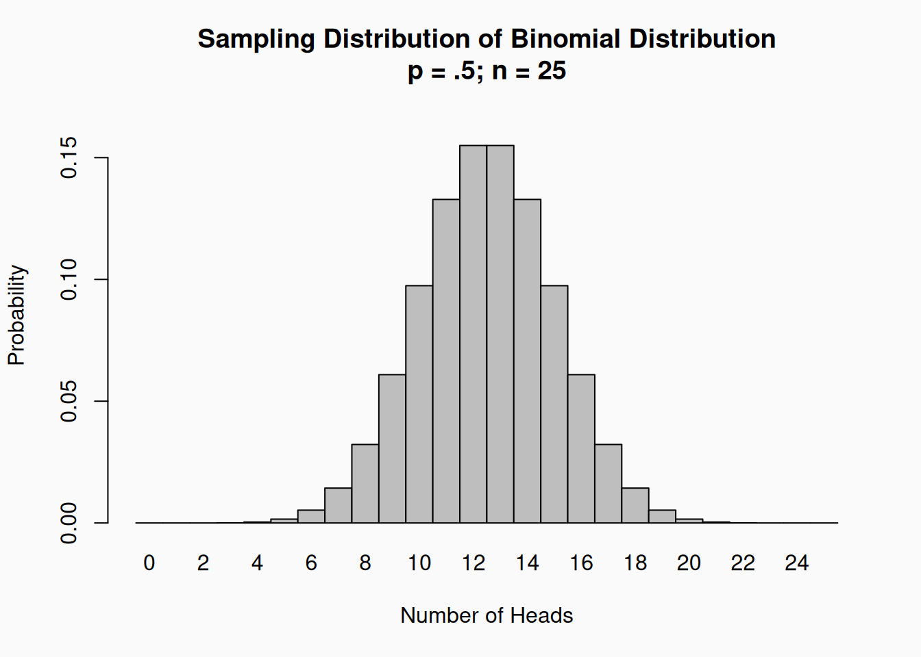
We usually express the null hypothesis as a particular value for a statistical parameter. For example, consider coin flips. We can model coin flips as a binomial variable drawn from a binomial distribution: $\sim \mathcal{Binom}(n, p)$. If the coin is fair that means that $p = .5$; This is the null hypothesis for a coin flip. Based on this null hypothesis, we can compute the distribution of coin-flip counts we’d expect to see, if we flipped a coin, say, twenty-five times:

We’d generally expect to see something like 12 or 13 out of 25 heads. However, even if the null hypothesis is true—$p = .5$—we would still expect to have samples where we get more (or fewer) heads sometimes.

Let’s say that we actually flipped a coin 25 times and measured 18 heads. In colloquial English we might say something like, “wow I flipped a coin twenty-five times and observed 18 heads. What are the chances?”. This colloquial expression is basically saying “if we assume the null hypothesis ($p = .5$) is true, what is the probability of flipping eighteen-out-of-twenty-five heads?” The answer is 0.014326. That’s pretty unlikely, right? We might, intuitively, start to think that maybe the null hypothesis is wrong…the coin might be biased!

Let’s consider another example, similar to what we’d see in real research. Imagine that I hypothesize that men enjoy heavy metal music more than women. To test this hypothesis, we’d need to come up with operational definition for “enjoy heavy metal.” We could then measure this variable in samples of self-identified men and women. We can model the relationship between gender (0 for women; 1 for men) and “metal enjoyment” using a simple statistical model like this:

\[ \text{metal enjoyment} = \beta_0 + gender * \beta_1 + \epsilon \\ \epsilon \sim \mathcal{N}(0,\,\sigma) \] We are assuming the “metal enjoyment” responses will be normally distributed around some mean value. If the null hypothesis is true, then $\beta_1 = 0$, which means that men and women have the same mean enjoyment ($\beta_0$). The research hypothesis would be that $\beta_1 > 0$, so the average enjoyment for men is higher than for women.

Let’s pretend we did this experiment, sampling 20 women and 20 men, and got these numbers in our sample:

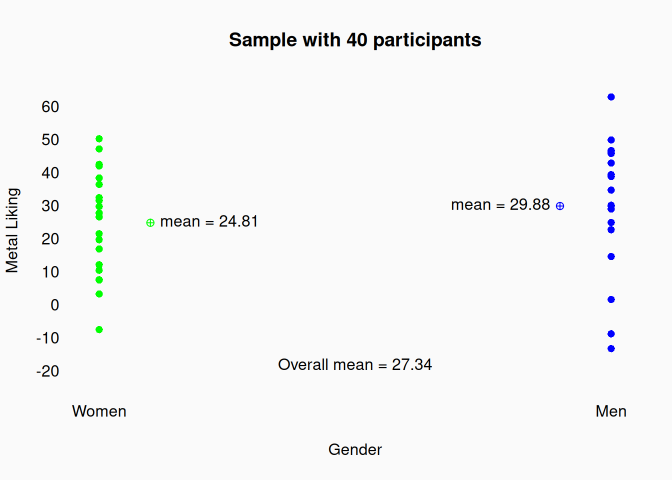
In this sample, the mean for metal enjoyment value for men is higher than the mean for women. In our equation, $b_1$ (the statistic for $\beta_1$) is $29.88 - 24.81 = 5.06$. That seems to be inconsistent with the null hypothesis. $5.06$ is clearly more than 0! However, even if the null hypothesis was true, we would still expect to see the two means being different in our sample just by chance. The question is, how likely is it that we’d observe $b = 5.06$ if $\beta = 0$? We need a sampling distribution for $b$!

Luckily, as we’ve learned, the central limit theorem tells us that sample means are normally distributed with the same mean as the population distribution and with a standard deviation of $\frac{\sigma}{\sqrt{n}}$. From this we can actually compute a sampling distribution for $b_1$.

The standard deviation of sample means (e.g., the standard error) is going to be $. What happens if we take the difference between two of these distributions? We learned in the “Model Fitting” lecture that a wonderful property of variance is that it is additive: $Var(x + y) = Var(x) + Var(y)$. Guess, what the variance of differences ends up being the same!: $Var(x - y) = Var(x) + Var(y)$. The variance of sample means will be the standard error squared: $(\frac{\sigma}{\sqrt{n}})^2 = \frac{\sigma^2}{n}$. If we assume that the standard errors of the two groups are the same, then we can conclude that the standard deviation of the differences will be: \[ \sqrt{\frac{\sigma^2}{n} + \frac{\sigma^2}{n}} = \sqrt{\frac{2\sigma^2}{n}} = \frac{2\sigma}{\sqrt{2n}} \]

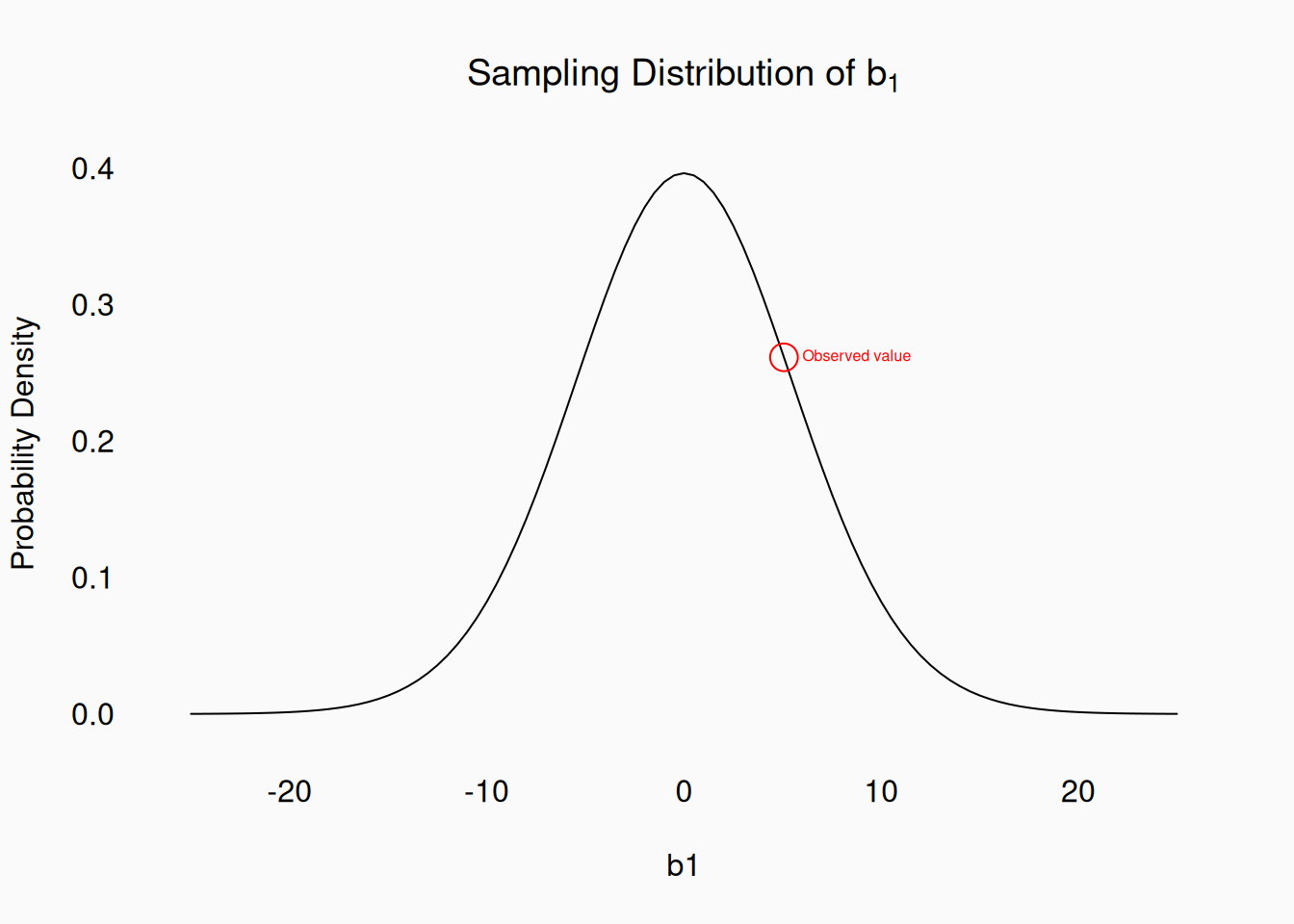
So, if the null hypothesis is true, the sampling distribution for the differences between two means with the same variance will be a normal distribution with a mean of 0 and a standard deviation of $\frac{2\sigma}{\sqrt{n_{men} + n_{women}}}$. So we can plot this sampling distribution and see where our observed sample ($b_1 = 5.06$) falls:

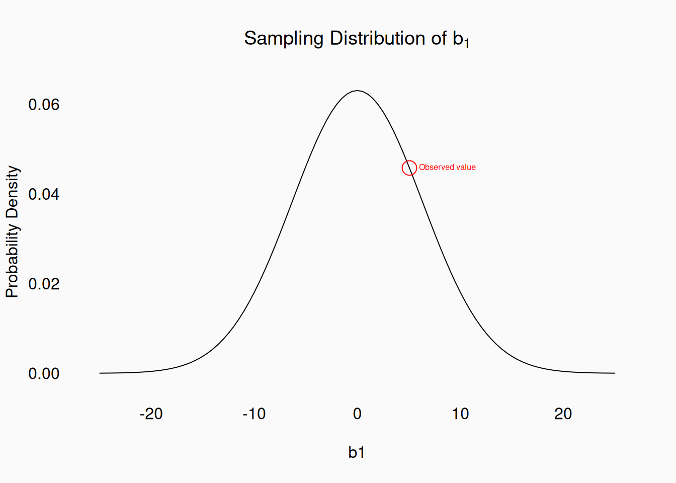
The probability density for $b_1 = 5.06$ is 0.0458. Note that we can only calculate this number by assuming the null hypothesis is true! It’s like the coin flip, where we assume its a “fair” coin.

t distribution

Unfortunately, this analysis isn’t quite good enough! Why? Because we don’t know usually know the population ($\sigma$) standard deviation. We can only calculate the sample standard deviation $s$. So we want $\frac{\sigma}{\sqrt{n}}$ but all we have is $\frac{s}{\sqrt{n}}$.

How does that affect our sampling distribution for $b_1$? Our estimated $s$ itself has its own random variability: in some samples it will be bigger than the true $\sigma$, in other samples smaller. As a result, the distribution of sample means (and differences between sample means) won’t actually follow a normal distribution. Instead, it follows a slightly different distribution, called Student’s t distribution. A $t$-distribution has an additional parameter, the degrees of freedom, corresponding to the sample size. When the degrees of freedom are small, the $t$ distribution has much longer tails than the normal distribution. As the degrees of freedom increase, the $t$ distribution approaches the normal distribution.

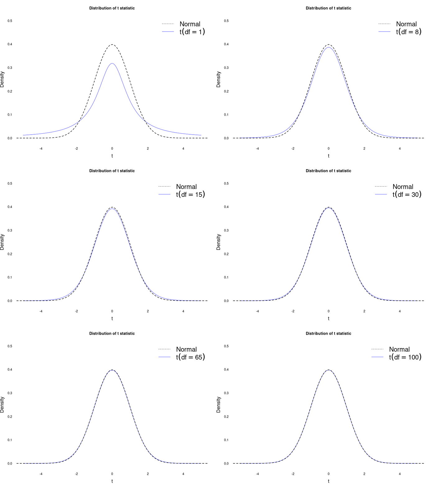
In our case, the null sampling distribution for the differences between two means, when estimating $s$, would actually be:

P values

In the previous section we calculated the probability of several different samples assuming a particular null hypotheses. For example, we saw that, assuming coin flip is a binomial distribution with $p = .5$, flipping 18 heads out of 25 has a probability of 0.014326:

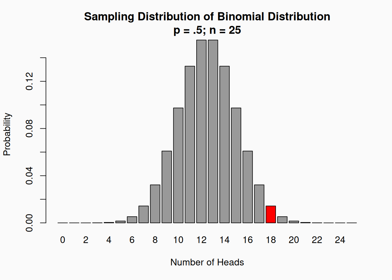
There is a problem here though: As your sample size gets bigger and/or the number of “levels” increases, the probability of any specific value will get smaller and smaller. For instance, if you flip a coin 1000 times—and assume that $p = .5$—the most likely outcome (500 heads) has a probability of only 0.025. If the sampling distribution is continuous (like the normal distribution), the probability (density) values will also get very tiny very fast.

The solution is that we don’t calculate the exact probability for the statistic we’ve observed. Instead, we calculate the probability for the statistic we’ve observed and all “more extreme” values, where “more extreme” means “a greater value in the direction of our research hypothesis ($H_1$)”. So for our 18-out-of-25 heads example, we’d sum up all the probabilities for 18, 19, 20, 21, 22, 23, 24, and 25 heads:

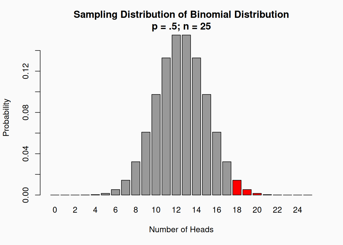
In this case, the probability-value sum for these levels is 0.0216.

In the case of our heavy-metal-liking sample, we’d look at the summed (actually integrated) probability for all values from 5.06–$\infty$.

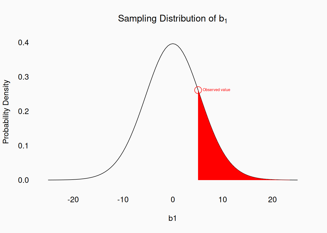
The integrated range of probability densities has a value of 0.185. These “observation and all more extreme values” probabilities are called: p-values.

Tails

Very often, our sampling distributions are symmetrical: just as the binomial, normal distributions, and $t$ distributions are. When calculating p-values, we must consider whether “more extreme values” includes both “tails” (sides) of the distribution. The question is, does the “direction” of the relationship we are inspecting matter to us?

With a coin-flip, we would probably by just as impressed by flipping 18 tails as 18 heads, right? Either case would conflict with the null hypothesis that $p = .5$ (i.e., that the coin is fair). We would thus treat this as a two-tailed test, and calculate a “two-tailed” p-value:

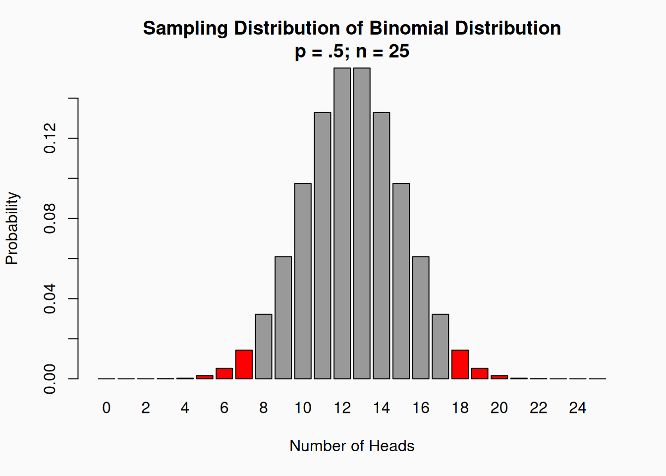
Our two-tailed p-value is actually $p =$ 0.0433, double the one-tailed p-value we calculated before.

In the case of our heavy-metal-liking sample (with $b_1 = 5.06$), I specifically hypothesized that men like heavy metal more than women. This is why I specified the null hypothesis as $\beta_1 > 0$. This is a one-tailed hypothesis; the other side of the distribution, where $\beta < 0$ (i.e., women like metal more than men), is not being considered. However, reviewers will regard one-tailed hypotheses with skepticism. Why? If our sample had found that women liked metal more than men, would we have discarded it? No, we probably would have reported it. We might have said, “Wow, we discovered that woman actually like metal more then men. What an interesting result!” This is why doing a two-tailed test is the default…in fact, using a one-tailed test without a very clear explanation is very likely to be questioned.

The two-tailed p-value for $b_1 = 5.06$ includes all values from -5.06–$-\infty$ and 5.06–$\infty$:

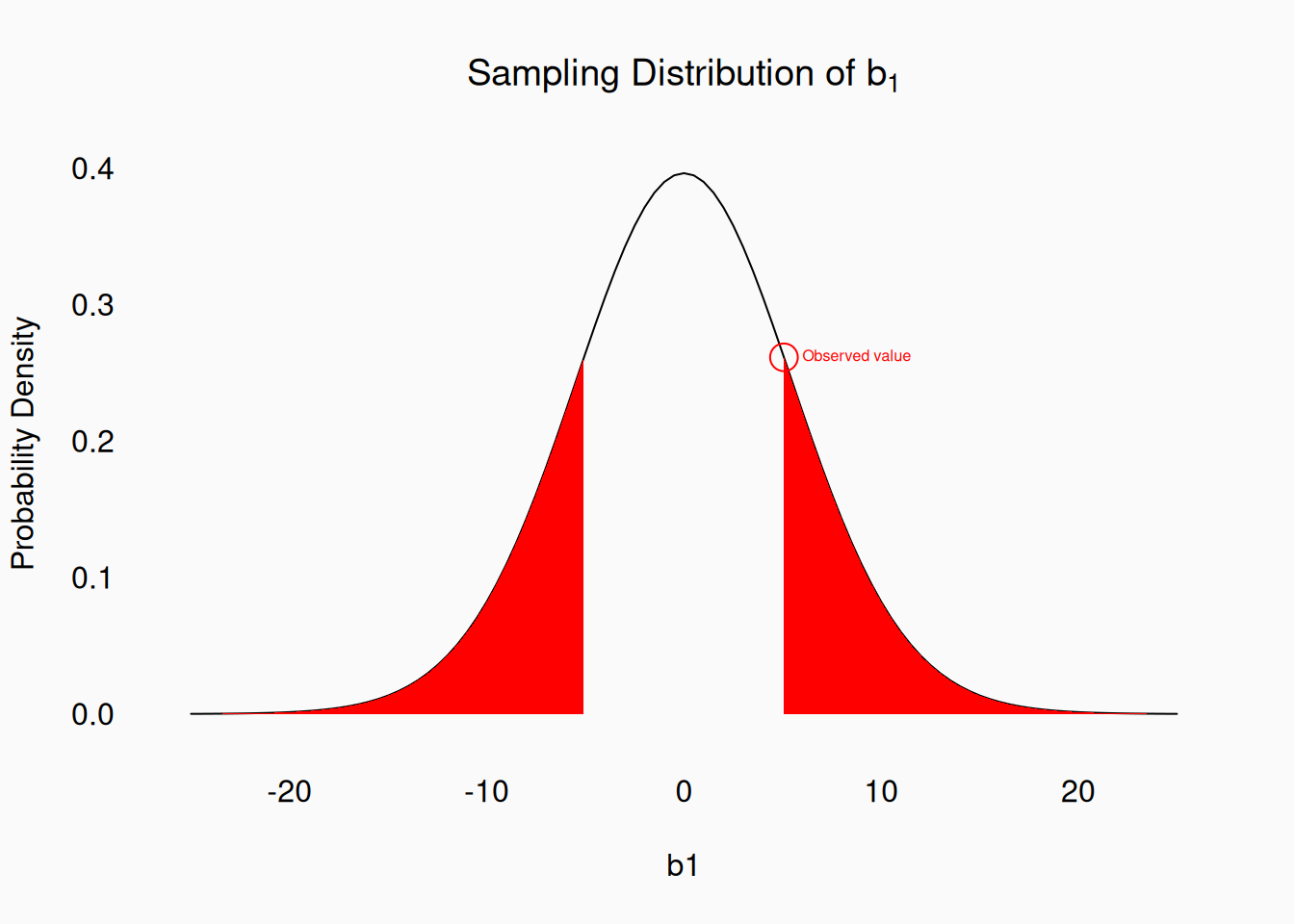
The two-tailed p-value is again double the one-tailed p-value: 0.1095.

Significance Testing

P-values are not the final product in a statistical test. The Null Hypothesis Significance Testing procedure uses p-values, but is more than just p-values! The full NHST procedure is as follows:

1 Select an “alpha level” ($\alpha$).
- The alpha level is a “cutoff” level—a line-in-the-sand that you establish a priori. The truth is that the alpha level has already been selected for you: $\alpha = 0.05$ is so standardized that any other alpha level will be viewed with suspicion.
2 Construct a statistical model and specify the null hypothesis (one or two-tailed).
3 Sample and measure data.
4 Calculate p-value, based on the null hypothesis.
5 Check, is the p-value, less than the alpha level?
- If $p < \alpha$, we can conclude that the result is “significant” because the null hypothesis is not consistent with the data. Since the alpha level of $\alpha = .05$ is standard, you will see papers frequently reporting $p < .05$ for “significant.”
- If $p \geq \alpha$, we conclude that the results are “not significant,” and we can’t reject the null hypothesis. In other words, it still seems plausible that the null hypothesis is true, and—as skeptical scientists—we conclude that the simpler null hypothesis is correct, and our hypothesis is wrong.

What is the logic of this procedure? The NHST is a procedure for the scientific community (as a whole) to limit Type 1 errors. A Type 1 error—also known as a false positive—occurs when we claim something to be true which is in fact false. Specifically, we don’t want to conclude that a hypothesis is true when in fact it is false. For example, I don’t want to conclude that men like heavy metal more than women if this is in fact false.

Let’s walk through it. First, lets assume that in some (many) cases, our scientific researchers like us investigate hypotheses that are wrong—in other words the null hypothesis is true. When the null hypothesis is true, 95% of our results will be correct non-significant results. However, even when the null hypothesis is true, 5% of our results will be significant ($p < .05$)—we’ll declare a significant result, consistent with our research hypothesis, and thus make a Type 1 error. However, the NHST procedure (with $\alpha = 0.05$) assures that Type 1 errors (across the scientific community) only make up at most 5% of “significant results.” Still, we know that up to 5% of studies which report “significant results” are wrong, so we remain skeptical, even of our own significant results.

Of course, not all our research hypotheses are wrong (or at least we hope so!). Sometimes the null hypothesis is false. In these cases, we can hope that all of our results will be significant ($p < .05$). In reality this is not the case: sometimes we’ll get non-significant results even when the null hypothesis is false. These are Type 2 errors—we claim that our hypothesis is not true, when it in fact is.

The chance of getting a significant result when the null hypothesis is false is called statistical power. Power depends on your sample size, as well as the strength of the effect. If, for example, men enjoy heavy metal a lot more than women, then it would be very likely that we’d get a significant result (high power). If on the other hand, men only enjoy metal a little bit more than women, it might be very hard to get a significant result, even though the null hypothesis is false ($\beta_1$ is small, but not zero). In these cases, we’d need a very large sample size to get enough power.

The NHST procedure basically ignores Type 2 errors—and is often criticized for it. However, this approach is motivated by general scientific skepticism: Since we know humans are biased toward finding what they want to find, we enforce rigorous skepticism on ourselves by focusing entirely on avoiding Type 1 errors. In general, reviewers will mostly be concerned about Type 1 errors. If you make analytical decisions which bias the result away from the null hypothesis, reviewers will be afraid that you are “inflating” the Type-1 error rate. On the other hand, if we make choices which are biased towards the null hypothesis, we say that these choices are “conservative’—they should be safe, because they won’t inflate Type-1 errors.

The $\alpha = 0.05$ level became the standard because it is a reasonable compromise between Type 1 and Type 2 errors. We, as a community, could lower our Type-1 error rate by using $\alpha = .01$ (we’d only expect to have at most 1% Type-1 errors). However, there is a trade-off: if you limit Type-1 errors, you will increase Type-2 errors—if we used $\alpha = .01$, it would be even harder to get significant results, even when the null hypothesis is in fact false.

Interpretating NHST

So, what does a “significant” result mean? This is, unfortunately, the most confusing part of NHST, because it is not intuitive.

A significant result does not mean the research hypothesis is proven true.
A significant result does not mean the null hypothesis is disproven.
A significant result does not mean that there is a less than 5% chance the null hypothesis is true.
- The p-value is computed by assuming $H_0$ is true, so it can’t be a measure of whether it is true!

So how do we interpret significant results? If the null hypothesis is true, there’s at most a 5% chance we’d observe this result. So you can say something like there’s at most a 5% chance that we are making a Type 1 error.

What does a “non-significant” result mean? Many will argue (including Fisher, who invented it) that “failure to reject the null hypothesis” is not evidence in favor of the null hypothesis. Basically, that a non-significant result is inconclusive. Unfortunately, that would mean that we never find evidence against our research hypotheses. We have to consider “failure to reject the null hypothesis” as evidence against the research hypothesis…or else nothing could ever be falsified!

Interpreting P-values

Part of the confusion with NHST arises is because we tend to get too hung up on the actual p-values. The p-value is not the significance test. The significance test is the whole procedure outlined above. In fact, p-values are actually very poor statistics by themselves.

It is tempting (and all too common) to interpret p-values as a measure of effect size:

“A small p-value ($p < .0001$) means the predicted effect is strong.”
“A larger p-value ($p = .045$) means the predicted effect is weak.”

Basically, we are treating $p$ as a descriptive statistic. However, the magnitude of the p-value is determined as much by the sample size as the effect size. Thus, this is a bad practice.

To summarize, $p$-values are bad descriptive statistics. ($p$-values are not inferential statistics at all!) P-values are used as part of a NHST, but they are not the whole deal. So when you think to yourself

“isn’t a p-value of 0.06 just about the same as a p-value of 0.04?”
“Why does an arbitrary cut off matter?”

You are right! (And you are not the first to think this.) A $p$-value of .04 is meaningless and a $p$-value of .06 is also equally meaningless.

However, the actual p-value doesn’t really matter. If $p = 0.051$ the result is not significant. If $p = 0.049$ the result is significant. This may seem crazy, but it is necessary to assure that, overall, we as a community cap our Type 1 errors at 5%.

If everybody says “0.051 is close enough, lets call it significant,” then our Type 1 error rate will actually be 5.1%…and you can imagine how things would creep up. Maybe $p = 0.075$ is close enough right? Woops, now our Type 1 error rate is 7.5%.

There is also a bad habit (in my opinion) among some researchers of reporting p-values between 0.05–0.10 as being “marginally significant.” This flies in the face of the NHST logic. Conversely, it is pretty much standard that people will report very small p-values as $p < .01$ or $p < .001$ or even $p < .000001$, and call them “highly significant.” But they didn’t pick those alpha levels in advance (a priori).

Reporting

The best practice for reporting a NHST is along these lines:

If $p < .05$
- “The result is not consistent with the null hypothesis.”
If $p >= .05$
- “We cannot reject the null hypothesis.”

However, the NHST is just the basic starting point for the analysis and report. You should report the effect size (usually with graphs). If you have a coin that is biased to $.51$, it might be statistically significant, but its not really practically significant. You may also add some additional, post hoc analyses, where you dig into details of the data more after the a priori NHST.