45  Describing data

(Modified on 2026-08-11)
4,342 words

Warning: Previous request to
`use_python("/home/nat/.virtualenvs/r-book/bin/python", required = TRUE)` will
be ignored. It is superseded by request to `use_python("/usr/bin/python3")
Warning: The request to `use_python("/usr/bin/python3")` will be ignored
because the environment variable RETICULATE_PYTHON is set to
"/home/nat/.virtualenvs/r-book/bin/python"

Once you collect some data—either by collecting it yourself or accessing an existing dataset—the first step should always be to get to know the data.

This process is important so that you understand what information is available in the data, what isn’t available, and to identify problems in the data.


You need to know your data so you can make appropriate analysis decisions and conclusions. You also need to know your data so you can make arguments about data validity. Does the data match the theory/construct? Do the relationships in the data match the theory/model? It is also essential to communicate important features of your data to your readers. If there are problems in the data, you need to find and acknowledge them so you can improve your analysis and/or preempt criticism.

Inspecting Data

Generally, you just want to be familiar with the data overall. However, there are also specific problems you should look for:

  • Errors
  • Inconsistencies
  • Undocumented/unknown content

The main thing you want to look out for is error in data. There are always errors in data—often, lots of error; Even in widely-used, peer-reviewed, datasets. Even if you gathered your own data, I guarantee that you will (sometimes) make mistakes which introduce error in your data. It could be a typo in a script, or a problem in an experimental interface you designed or an algorithm you wrote.


For our “tempo stability” paper (2024), we worked with a sample of $$50,000 songs from the Spotify API. On inspecting the data, we found numerous errors: For example, hip-hop songs that were (supposedly) released in the 1920s and songs with negative tempos! These sorts of errors may, or may not, bias or otherwise affect analysis results. They might also lead to bugs in your analysis code: for instance, if you try to take the logarithm of a negative number (as I did, when there were negative tempos in the data), you’ll get an error or a missing value which can propagate to future errors.

Spot Checking

It is essential to spot check your data: By this I mean, actually look directly at specific pieces of raw data. This might mean inspecting text files in an editor, or listening to audio files. For anything but the smallest dataset, it’s not feasible to check all the data, so instead look at a random sample. For example, if you have a large sample with thousands of .XML files, randomly inspect at least a few dozen. This will help you find problems and understand the data.

The next thing you should do is spot-check any outliers—values that don’t seem to match the rest of the data. For example, in my tempo-stability dataset, I calculated the mean and standard deviation of tempo estimates in each track in our sample, and plotted these. By looking at these means, I was able to find tracks that had crazy low mean tempos (like \(20_{bpm}\)). I then went and looked at the data for those tracks and discovered the negative tempos I mentioned above. I also noticed some outliers with regards to standard-deviation as well; When I checked those outlier tracks, I found that the standard deviations seemed to be correct (the songs really had widely variable tempos).

Aggregate Checking

It is often impossible to inspect all your raw data. Instead, you can try to get aggregate information about the data and check that the aggregates make sense.

With most categorical data variables, even when there are millions of actual data points there are a much smaller number of unique values/levels. Try to list and inspect all the unique values that occur: for example, if you are working with a dataset of harmonic (chord) labels, you should look at all the chords that appear. You might expect to see labels like "C major" or “Ab minor"; However, on inspecting your data you might also see tokens like "C mjor", "K minor", or "Error: list index outside range" snuck in there! Hopefully, there are no more than a few hundred values which you can scan through fairly quickly—even a few thousand unique values can be scanned in an hour or two. (It helps a lot to sort the unique values alphabetically.)

For numeric variables, look at descriptive statistics, especially the range of the numbers. In most cases, you know (theoretically) what the range of values should be: For example, if you are working with MIDI note-number data, you probably shouldn’t see any values below 20 or above 90 (and even these are extreme), and certainly not -10 or 120.

Often ostensibly numeric data will have a few non-numeric character strings stuck in there, as well, so look out for problems like:

                BPM Genre
1  77.4223320954479   Pop
2  63.8950038305484  Rock
3  90.0792457954958  Jazz
4  149.616370245349   Pop
5  109.396001351997   Pop
6  105.229823633563  Rock
7  90.4978871368803  Rock
8  86.8435793789104  Jazz
9  115.234674985986  Rock
10 147.994559593499   Pop
11 102.978498525918  Rock
12 113.061804031022  Rock
13 85.3152309707366  Rock
14             Rock  <NA>
15 92.9134885361418   Pop
16 114.919225224294  Jazz
17 86.4231654745527  Jazz
18 89.3658999656327   Pop
19 113.228870783933  Jazz
20 149.039762760513  Jazz

Even when there is no “errors,” there can be inconsistencies in datasets. For example, you might see some chords labeled "C major" and others labeled "C maj". When you run statistics or an ML model, these two labels will “look” like two different chords, when they are really the same chord.

Data may also have surprises that aren’t “errors,” but aren’t well documented. For example, in an existing dataset of harmonic chord labels, the creators may have decided to label passages where no instruments are playing (so there is no chord) as "X" or "No chord", but failed to mention this in their documentation. Similarly, people are often confused to see "C64" as a roman-numeral chord label in Johanna’s Devaney’s TAVERN dataset (2015)—representing “cadential 6/4” chords—even though these are documented in her paper.


You can also check for construct validity issues. If you are looking at timing data, always try to suss out what the true sample rate was. For example, consider some hypothetical timestamp (in seconds) data, like:

 [1]  3.667 14.292 17.042 18.000 18.250 20.083 22.500 30.125 31.500 32.083
[11] 32.542 33.958 35.875 40.958 45.583 46.042 47.875 49.792 51.375 56.542

Looks like continuous timestamps right? Actually, these values are rounded to 1/24 (24 samples per second)—so the data isn’t quite continuous at all.

Visualization

Excellence in statistical graphics consists of complex ideas communicated with clarity, precision, and efficiency. … Graphics reveal data. Indeed graphics can be more precise and revealing than conventional statistical computations.

— Edward Tufte (1973)

The best way to describe data is to visualize the data—in a chart, graph, or plot. Graph distributions (all data points); Graph descriptive statistics; Graph relationships between variables.

The words “graph,” “plot,” and “chart” are often used as roughly synonyms. However, they have slightly different meanings. A graph shows lines (usually, a mathematical function), a plot shows points, and a chart shows other pictograms/shapes (like bars or pies). In a paper, they are referred to as figures.

Visualization serves two roles: 1) helping you understand your data and 2) as a part of the rhetorical process, showing your readers relationships and facts about the data that are relevant to your argument.

Get the Gist

When visualizing data, your goal should not be to communicate exact data values or statistics. Rather, your goal should be to convey the gist of the data. If you think it’s important to communicate specific values for some reason, tell them in a table, in your text, or in an appendix! That’s not what visualizations are for.

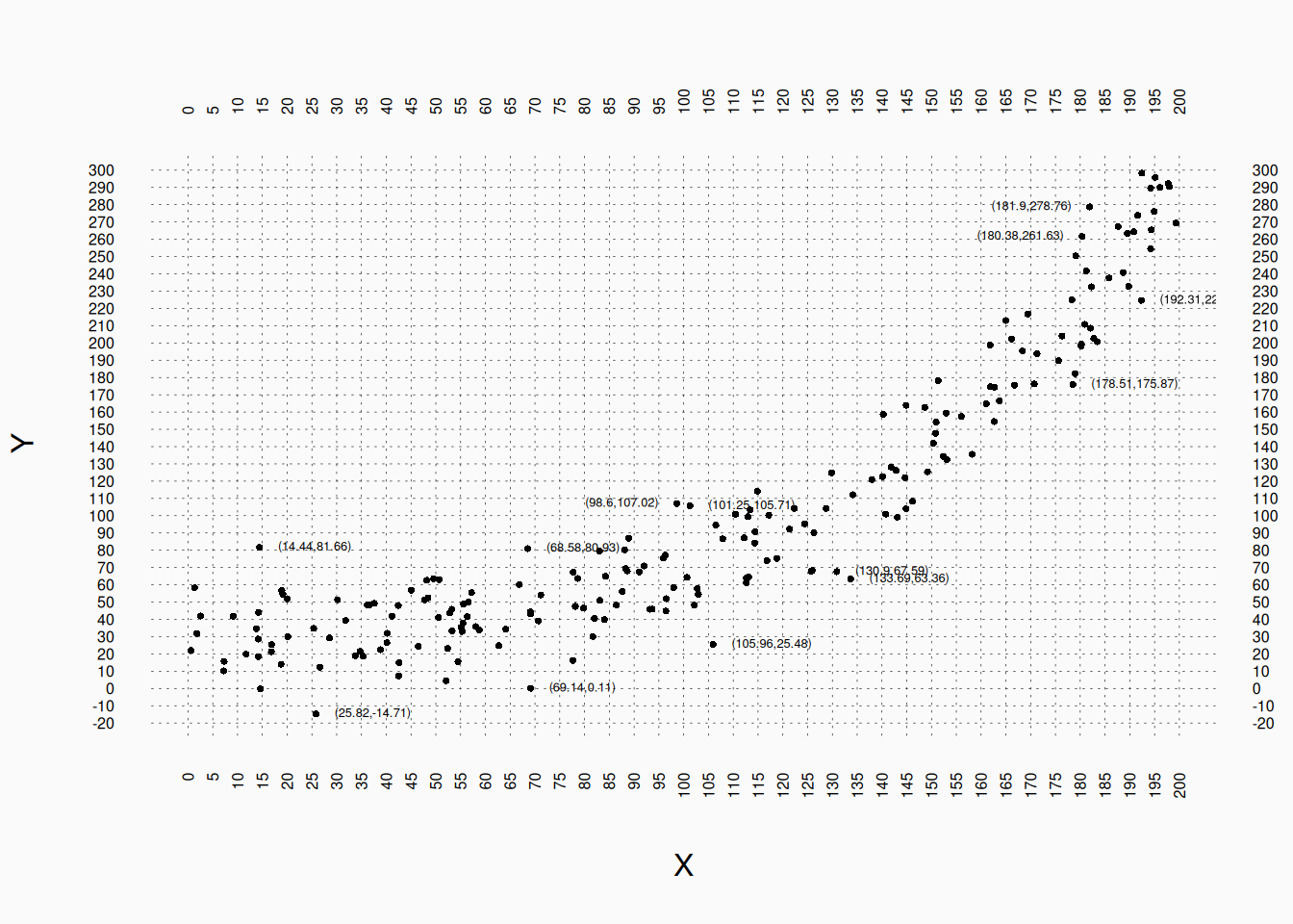
For example: don’t do this:

Having these (painfully) dense grid lines allows us to identify pretty precisely the value of every point—but why? What helpful information does it convey to our readers? I call this graphical overfitting: paying too much attention to the details of our data, rather than the underlying patterns we are actually interested in.

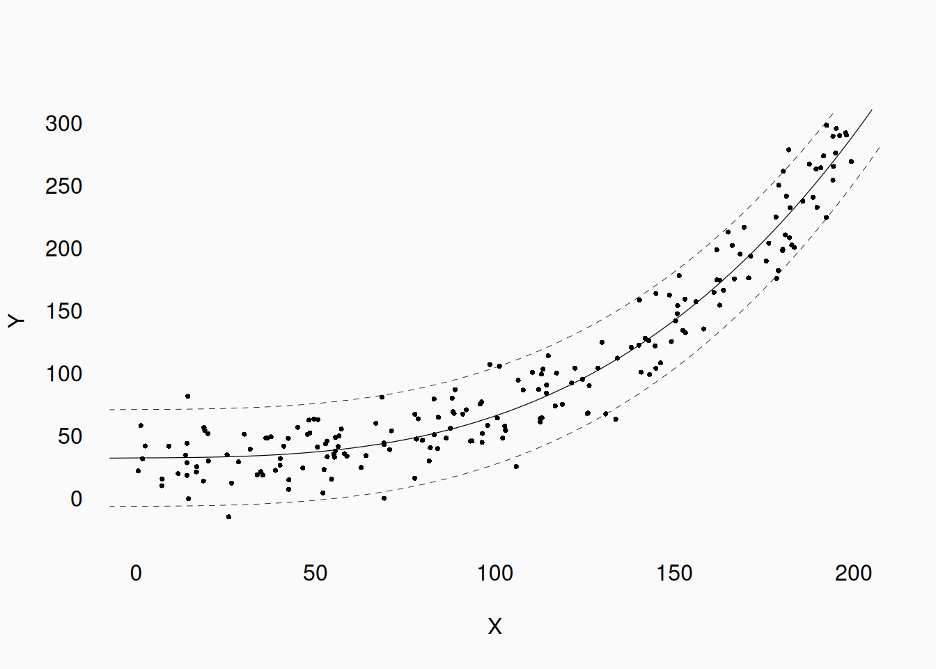
We (generally) want to use our data to make generalizable inferences, and our graphs should focus on showing the patterns that we would want to generalize about In this case, the useful patterns that we care about are:

  1. There appears to be a curvi-linear relationship between X and Y.
  2. The random error (in the Y axis) appears to be symmetrically distributed, somewhat tightly around the line.

This information is what our research claims would focus on, and this is what our graphs should focus on too. In contrast, the number of data points (in our sample) that happened to fall in the grid between \((75, 40)\) and \((80, 50)\) is not relevant. (If it ever is relevant for some reason, put it in a table.)

Let’s try again:

Much better!

Anscombe’s Quartet

One of the classic demonstrations of how important visualizing data can be is (Francis) Anscombe’s quartet (1973):

These four graphs show a two-dimensional data set with essentially identical descriptive statistics: In each graph, the mean of X, mean of Y, variance of X, variance of Y, and the correlation between X and Y are (almost) identical. Only by visualizing the data can we see that the datasets are totally different!

Standard Plots

The appropriate visualization for data depends on the nature of the variables, and the number of variables you are trying to visualize.

  • One variable
    • Categorical:
      • Bar plot
      • Pie chart
    • Numeric:
      • Histogram
      • Quantile plot
  • Two variables
    • Categorical:
      • Bar plot
      • Heatmap
    • Numeric:
      • Scatter plots
      • Line graph
  • Three variables
    • Categorical:
      • Bar plot(s)
    • Numeric:
      • Scatter plot(s)
      • Perspective (plane) graphs

One Dimension

Categorical data

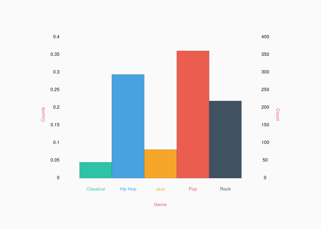
When working with categorical data we generally simply count the number of occurrences of each category and make a table. We can visualize such a table as a bar plot.

The information in any bar plot can always be conveyed to your readers in a table instead:

Genre Count
Classical 45
Hip Hop 294
Jazz 81
Pop 361
Rock 219

However, bar plots are more effective at conveying gist of the data. For example, is the count of Hip Hop closer to Pop, or Rock? It’s much easier to see (quickly) in the graph, compared to the table.


In a bar plot, the height of bars may indicate the actual counts of each level or the proportion of the total data in each level. In the graph above, I get the best of both worlds by showing proportions on the left and counts on the right.

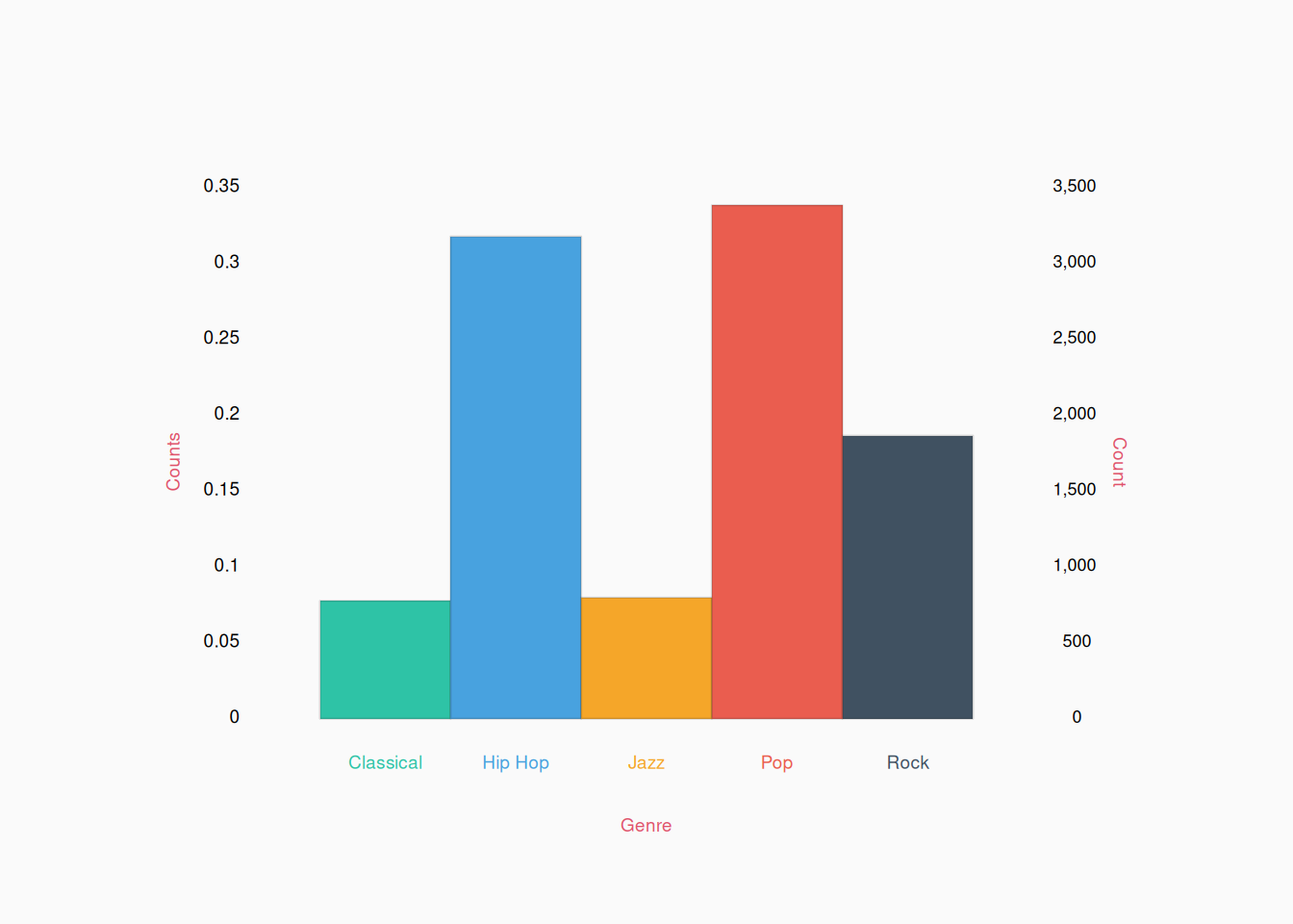
The advantage of counts is that they convey the total size of the dataset, where as proportions (a more abstract, quantitative measure) hide this information. Proportions also make more assumptions, as they assume that you have counted all relevant categories (so the proportions must sum to 1). On the other hand, proportions are easier to compare across datasets. For example, if we found another data set of genre labels that looked this:

If we look at the counts (on the right), we can see that this dataset is much bigger than the last one. However, by looking at the proportions (on the left), it is easier to see that, for example, the proportion of classical music is about the same as before.


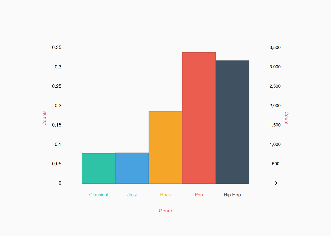
Bar plots are most useful when the total number of levels is fairly small (perhaps, 12 or fewer). In these (ideal) cases, each bar should be labeled with its own category. By default, the bars should be ordered in a meaningful way based on the levels of the variable, not the values of the barplot. We might organize labels alphabetically, as I do above, or perhaps group them based on some logic relevant to our research theories. For example, these categories might make more sense grouped musically like:

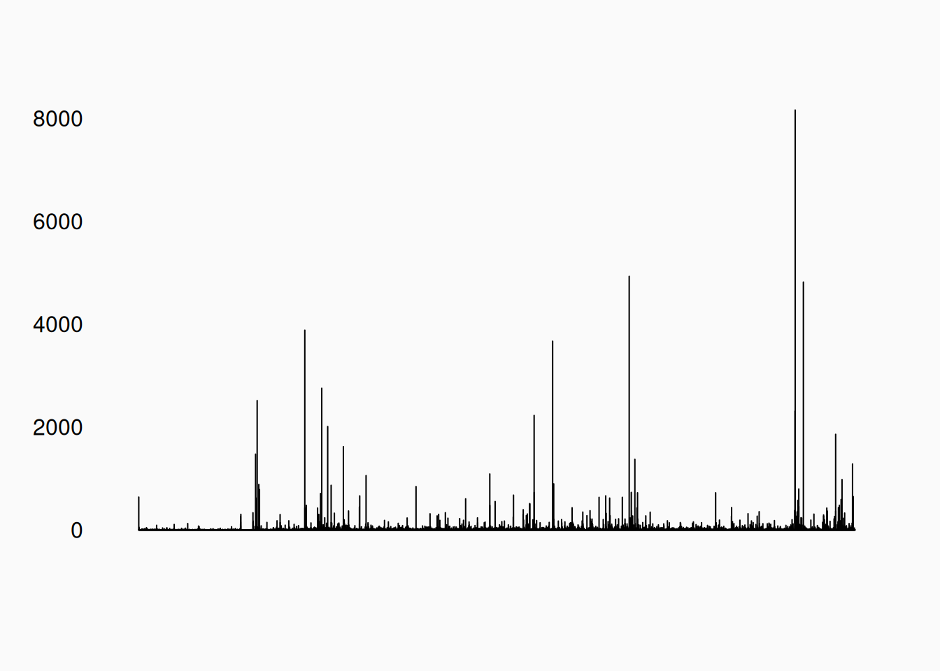
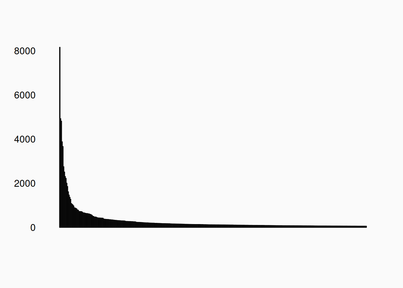
If there are a large number of categories (like more than 15–20), don’t bother labeling each bar. In these cases, bar plots are not really very useful; However, sometimes sorting a large numbers of bars by bar height can reveal useful patterns. For a classic example, let’s consider what happens if I count how often every unique “word” occurs in this text book. There are 196,016 in the book, but only 19,420 unique words. That is, we have sampled 196,016 values from a categorical variable with 19420 levels. A bar plot with this many levels, with the levels sorted alphabetically, will look like this:

Useless! However, if we sort the table by count, we see this:

We can now see that there are a small number of very common words, but that the frequency of words drops off exponentially.

  1. The most common word is “the,” occurring 8,164 times;
  2. The second most common word is “of,” occurring 4,930 times;
  3. The third most common word is “of,” occurring 4,930 times;.
  4. etc.

This is consistent with Zipf’s Law, which is often seen in this sort of data.


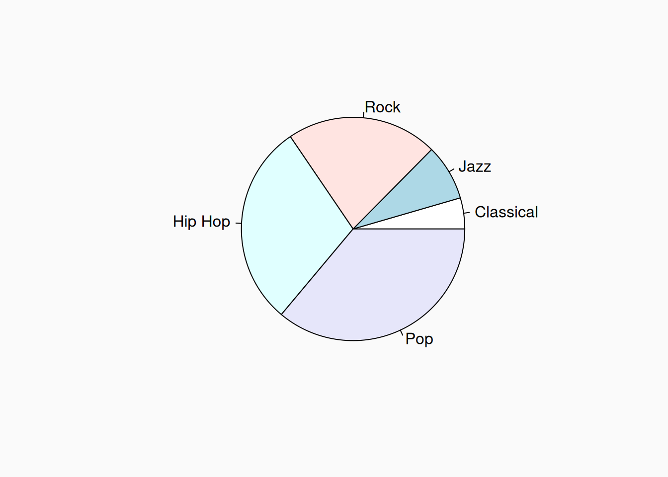
Another approach to graphing a single categorical variable is with a pie chart. Pie charts should be used sparingly, if at all, as they are looked down upon by many researchers. The issue is that humans have a hard time judging the relative size based on area:

How much more rock is there compared to jazz? Twice as much? Three times as much? It’s hard to judge. A bar plot makes this easier. However, a pie chart might be useful in certain cases, depending on what gist you want to point out to your reader. For example, it’s easy to see here that the dataset is about one third pop, one third hip hop, and one third other. This is not nearly as obvious in the barplots.

Numeric data

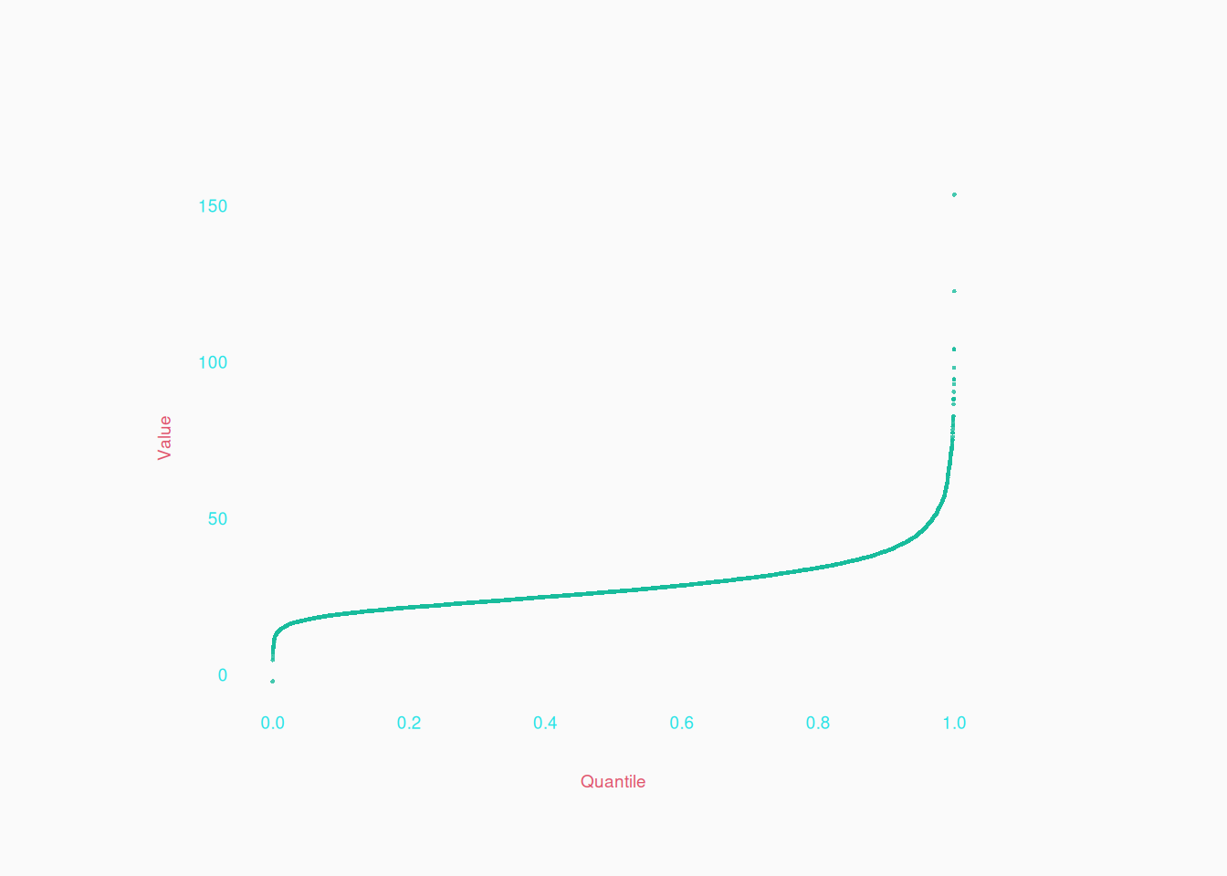
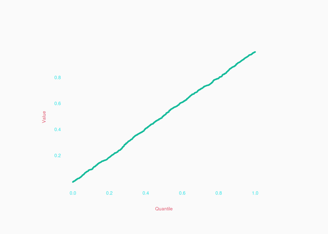
For numeric variables, the absolute best visualization is the quantile plot. Simply sort the data points, usually from lowest to highest, and plot them from left to right:

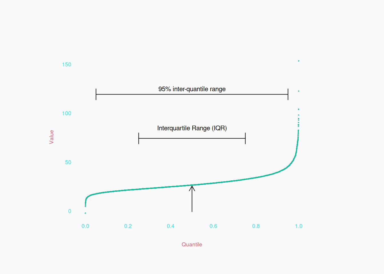
In such a plot, the X axis simply represents the quantiles of the data, with the median in the middle, and the quartiles at 25% and 75% of the screen, etc.

Quantile plots are extremely informative visualizations. From them, you can see useful “gists” like symmetry, the number of modes, and generally how concentrated data is at different Y values:

  • The flatter the curve is, the more concentrated the data is at the flat level.
  • The steeper the curve, the less concentrated.
  • The closer you are to \(45^{\circ}\)-angle curve, the more uniform the distribution at that point.

For example, here is a totally uniform distribution:

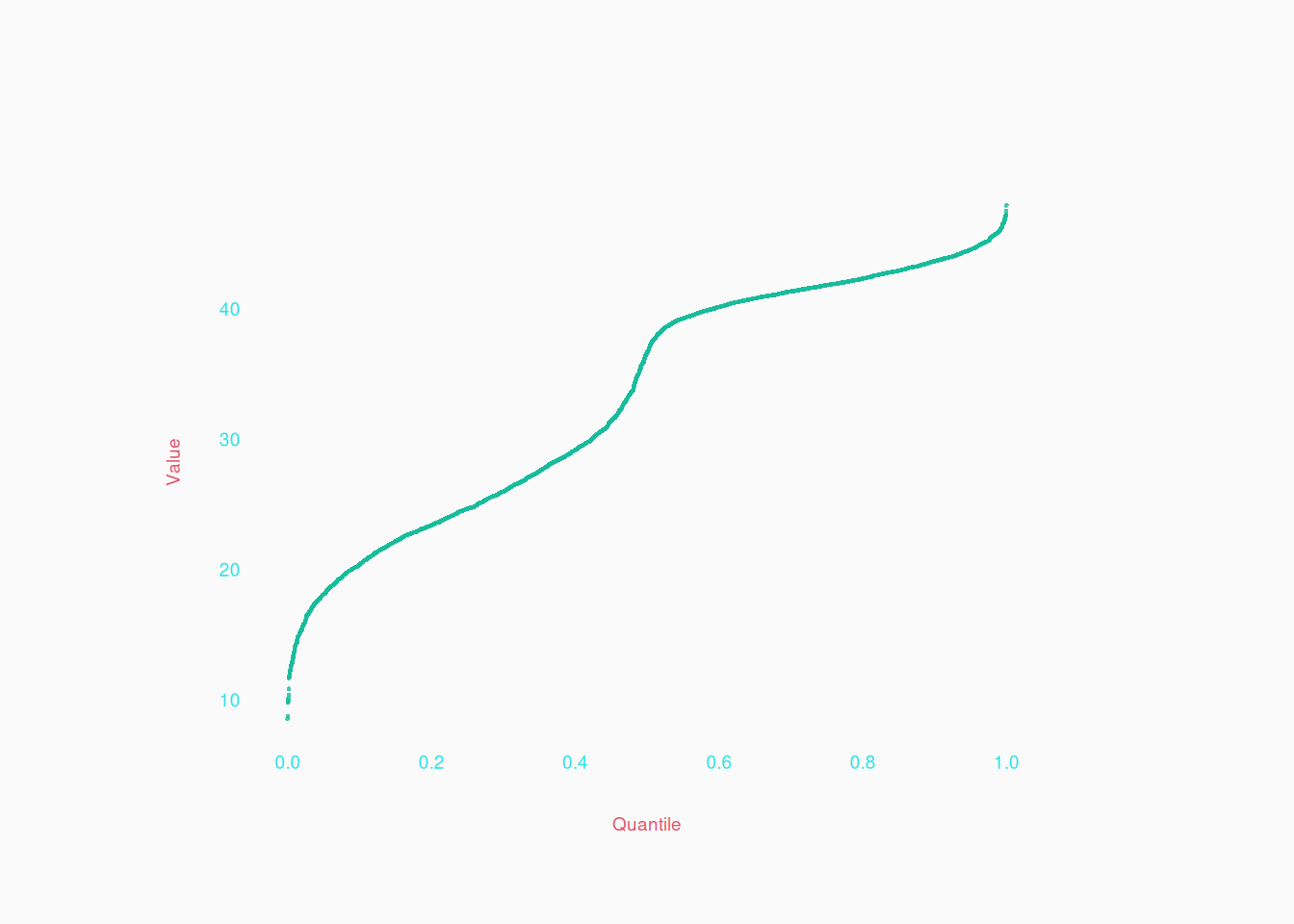
Here is a distribution with two peaks (bimodal):

Can you see which of the two peaks is more concentrated?

The upper one! We can tell because the slope is flattest where \(Y > 40\). The steep part in the middle is a relatively empty range between the two peaks.


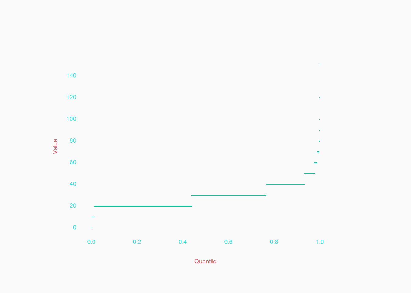
The really useful thing about quantile plots is that we are looking at all the data, so it’s also possible to notice small details about the sample (useful for descriptive analysis).

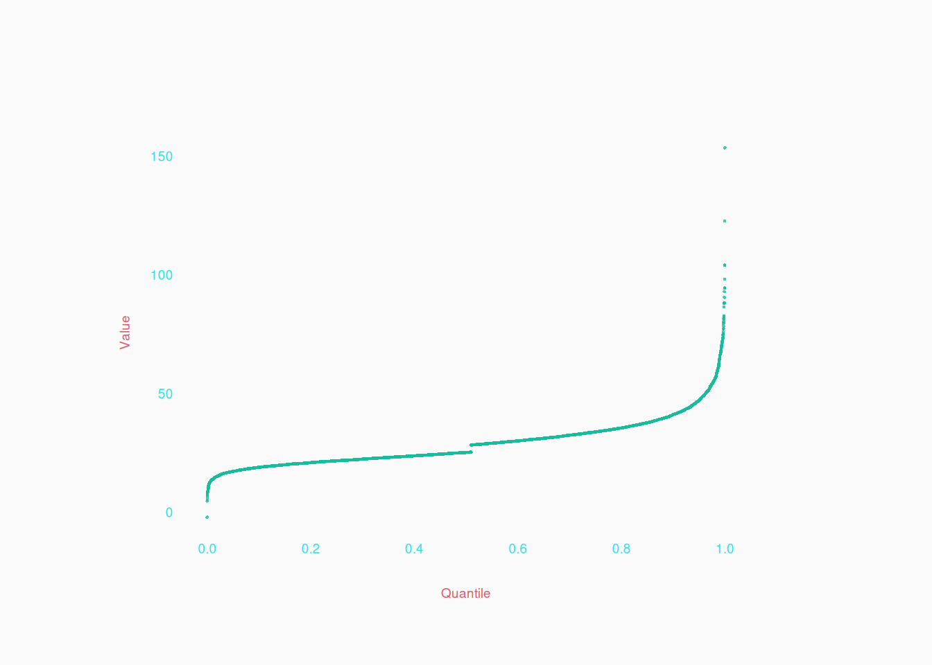
  • You can see how the most extreme individual values fit in the curve (bottom left, and top right points). Outliers will be obvious.
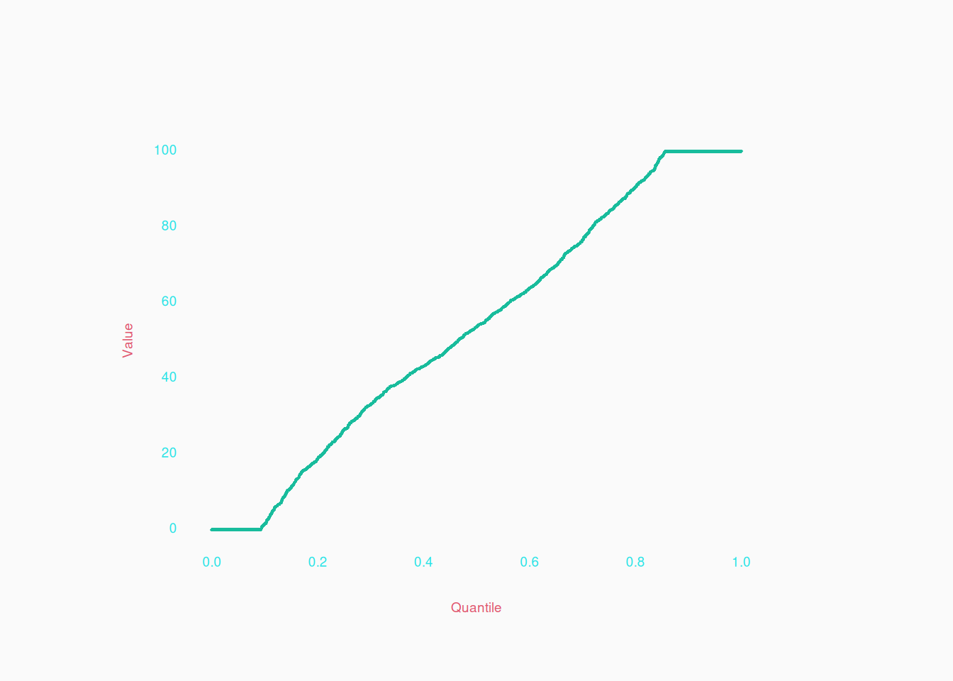
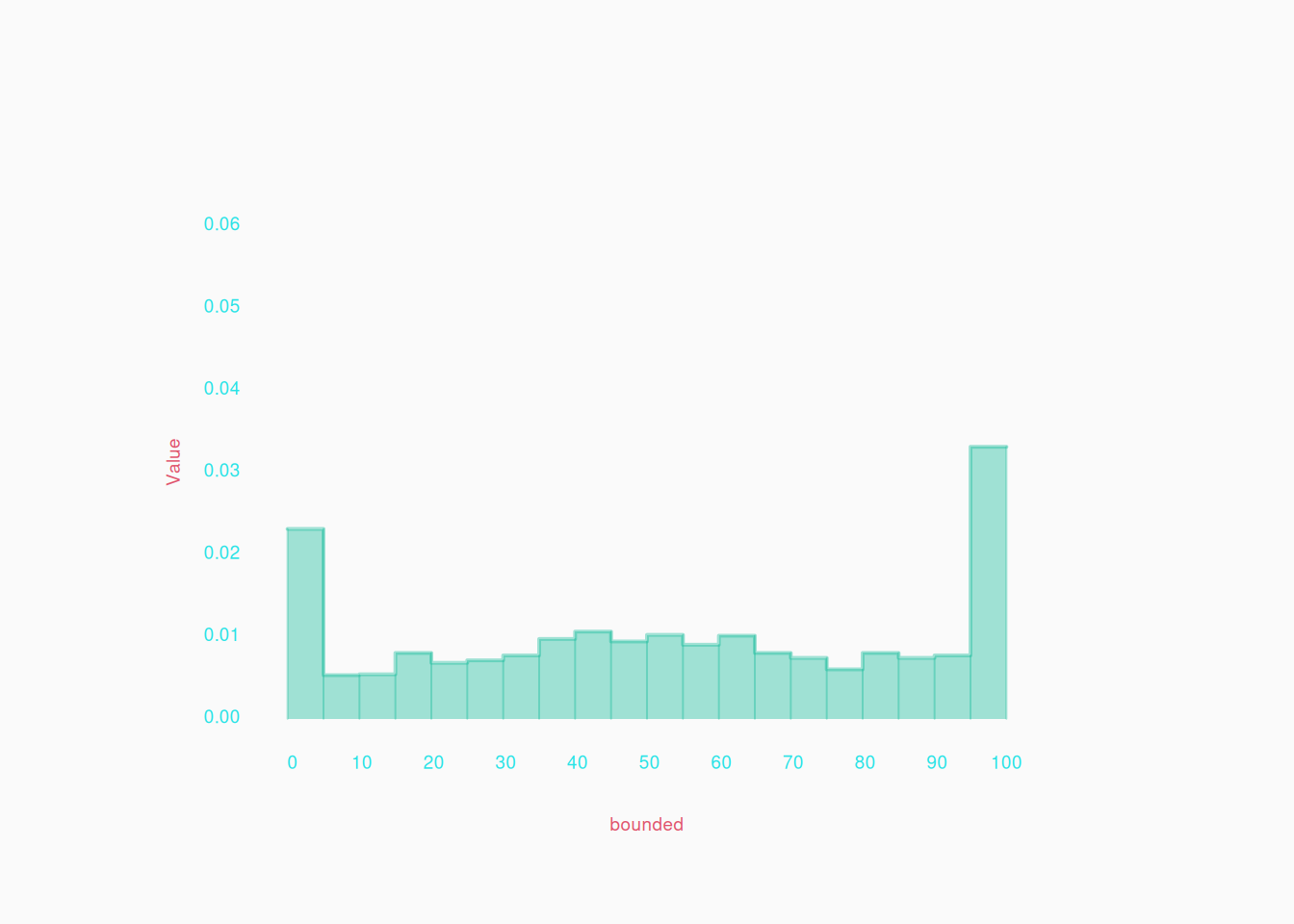
  • You can see where data values are bounded (example further below).
  • You can also see things like gaps, where no values occur, which show up as a break or a kink in the curve:


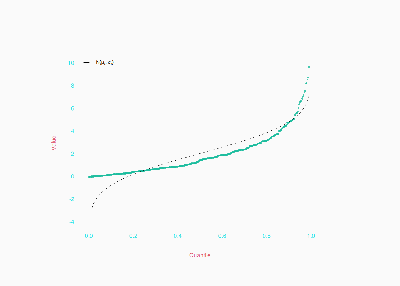
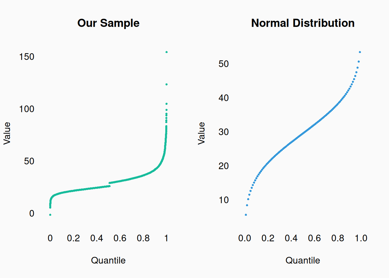
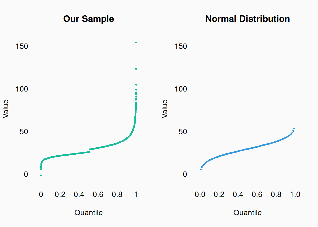
It is often useful to compare your quantiles to known distributions, like the normal distribution, shown here as a dashed line:


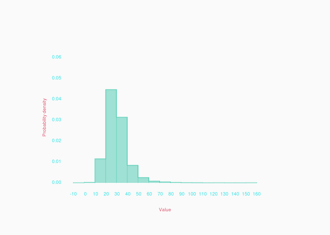
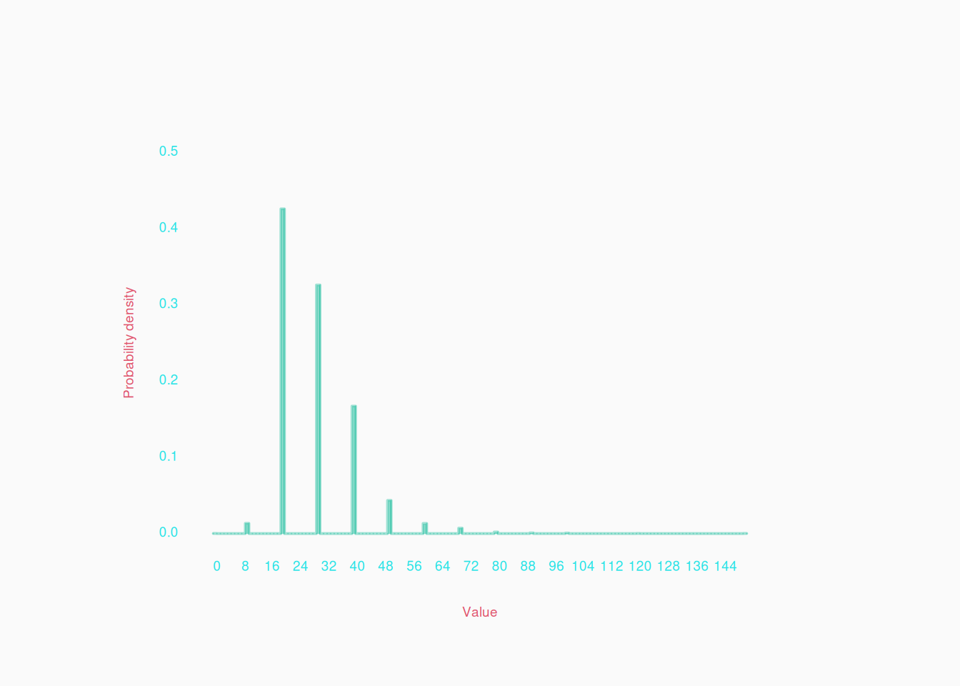
Another approach to visualizing a numeric variables, is with a histogram. Values of the variable are “binned” into ranges and the number of values in each bin are counted and then represented by the height of bars:

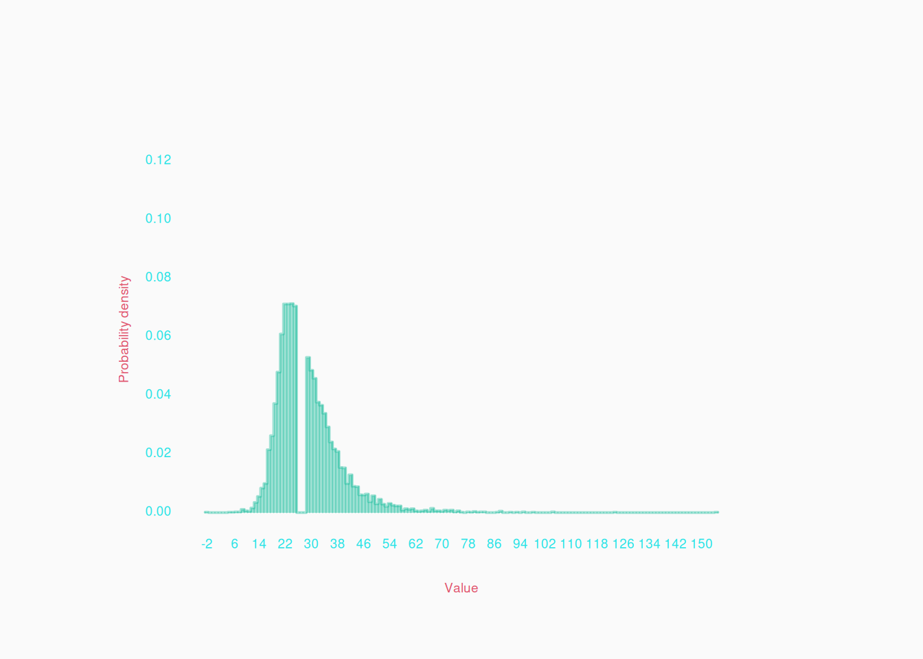
Histograms are more commonly seen in papers than quantile plots. However, they have one important disadvantage: the result depends a lot on the size of the bins. There are various ways of determining the size of bins, but it is generally automated by graphing software. Lets see what happens if we increase the number of bins on the same data:

Ah! Only now can we see that weird gap in the data, which we immediately saw in our last quantile plot.


Visualizing data in one dimension is extremely important during the data preparation and cleaning process! Use quantile plots and histograms to look for problems in the data, like the gap in the data shown above. For another example, you might wonder if a distribution is hitting boundaries:

Or perhaps a “continuous,” real-number variable is really being rounded more than you think:

This is where the quantile plot shines, because the histogram won’t show this unless there are a lot of bins.
Two Dimensions

We often want to visualize the relationship between two variables. This is necessary, for example, to visualize if they are correlated.

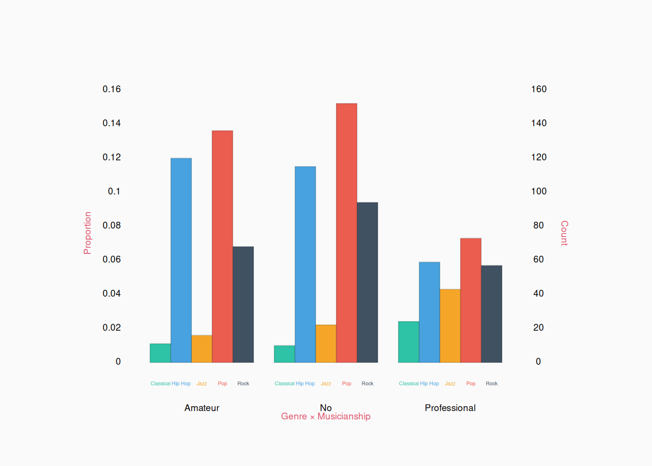
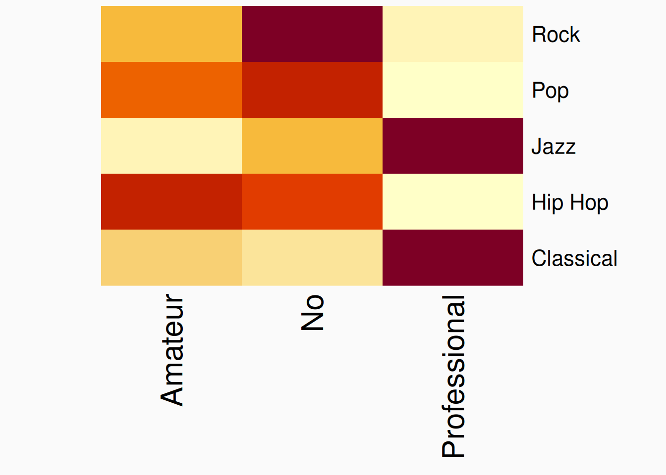
Two categorical variables can be counted up (or shown as proportions) in a two dimensional table. For example, maybe the genre variable from above could be paired with a musicianship variable:

           Musicianship
Genre       Amateur  No Professional
  Classical      11  10           24
  Hip Hop       120 115           59
  Jazz           16  22           43
  Pop           136 152           73
  Rock           68  94           57

For small enough two dimensional tables, we can effectively show this as a double bar plot:

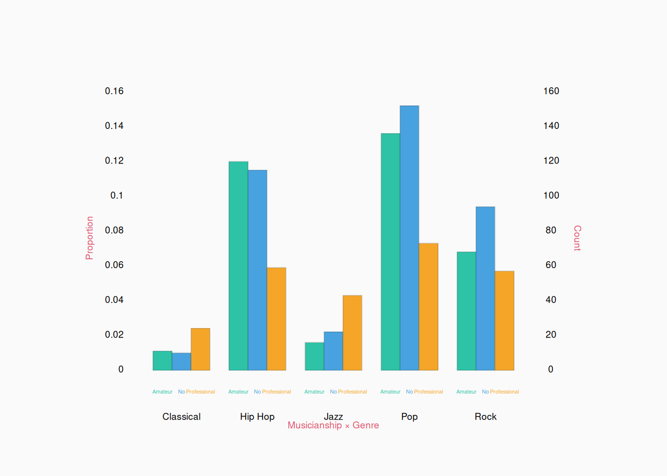
You can choose which variables to group together though. We can show the same data flipped:

The fact that each little cluster of bars has a different shape, shows that the two variables are correlated. (Classical and jazz genres are more likely to be professionals.)


If the number of categories is large (like more than ten), these sorts of bar plots become really hard to read. In these cases, I would simply show the table in a paper. An alternative is a heat map:

Heat maps are useful for large enough tables. However, color is much less effective at communicating numeric values, so bar plots or other visuals should be used when possible.

Scatter plots

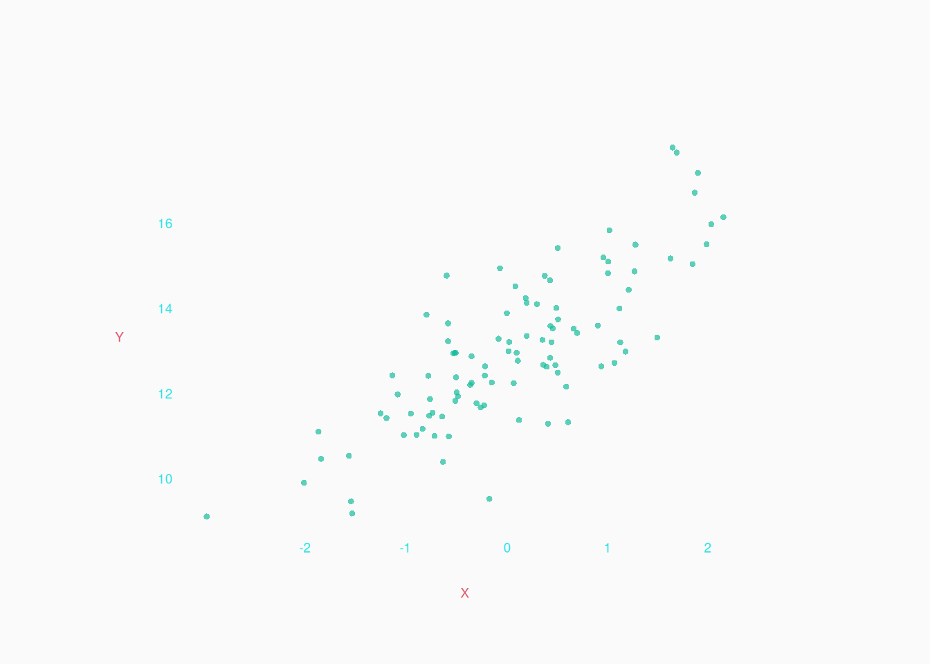
If working with two numeric variables (on integer/ratio scales), we can make the classic scatter plot.

Categorical X Interval

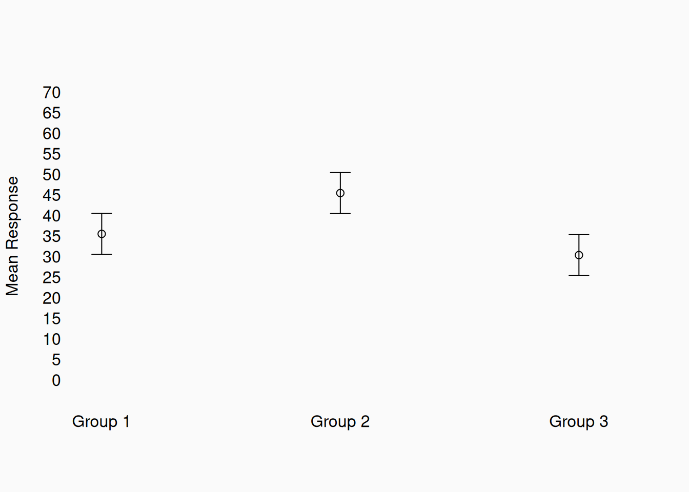
If one variable is categorical and the other numeric, it’s very common to plot group means, perhaps with confidence intervals:

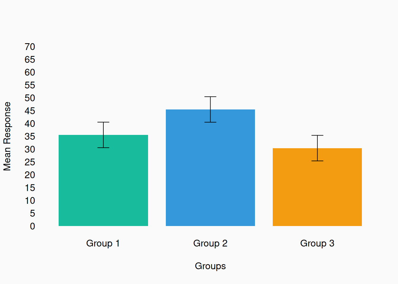
If the values are strictly positive (and ratio scale), you can use a bar plot instead.


Box and Violin plots

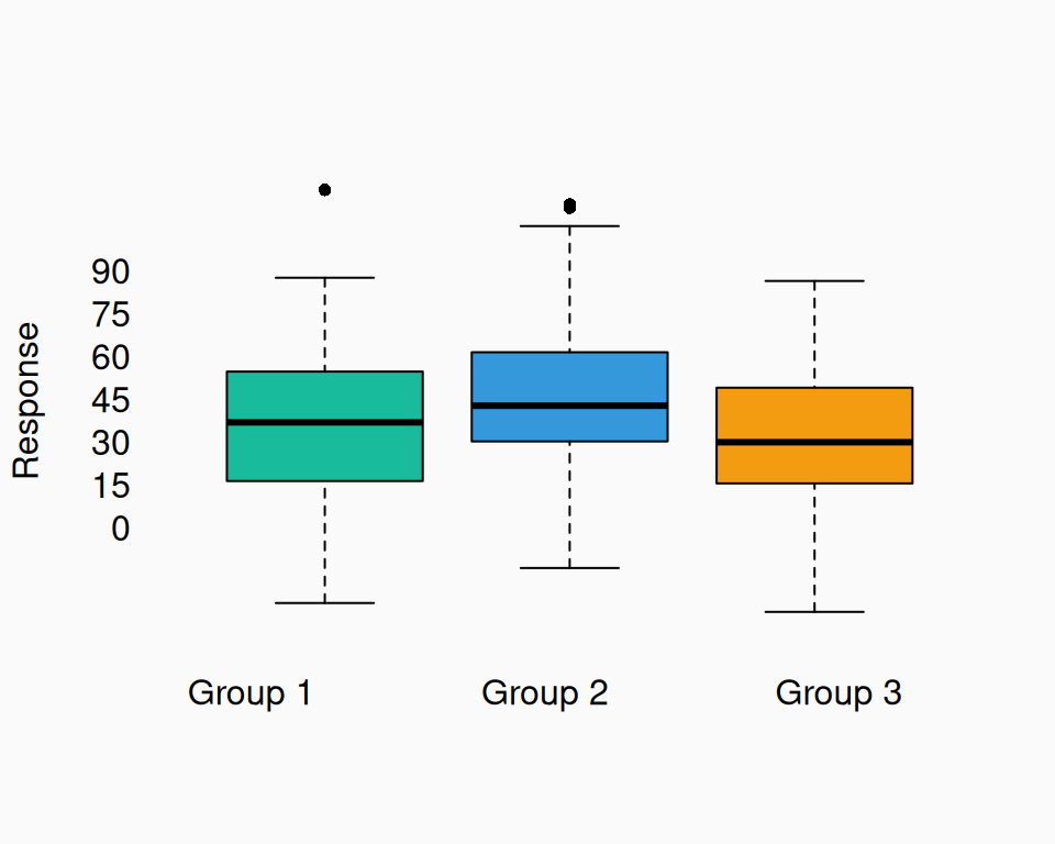
A box plot is a similar visual, which shows the distribution of numeric values within groups. However, unlike the plots above, a box plot shows more than just the mean:

I don’t like box plots because nobody knows what they actually represent! For example, people assume the black line is the mean, but actually:

  • The black line is the median.
  • The boxes are the 25%–75% quantiles (interquartile range).
  • The whiskers mark the 2.5%–97.5% quantiles (95% interquantile range).
    • Any values outside the 95% range are shown as individual points.

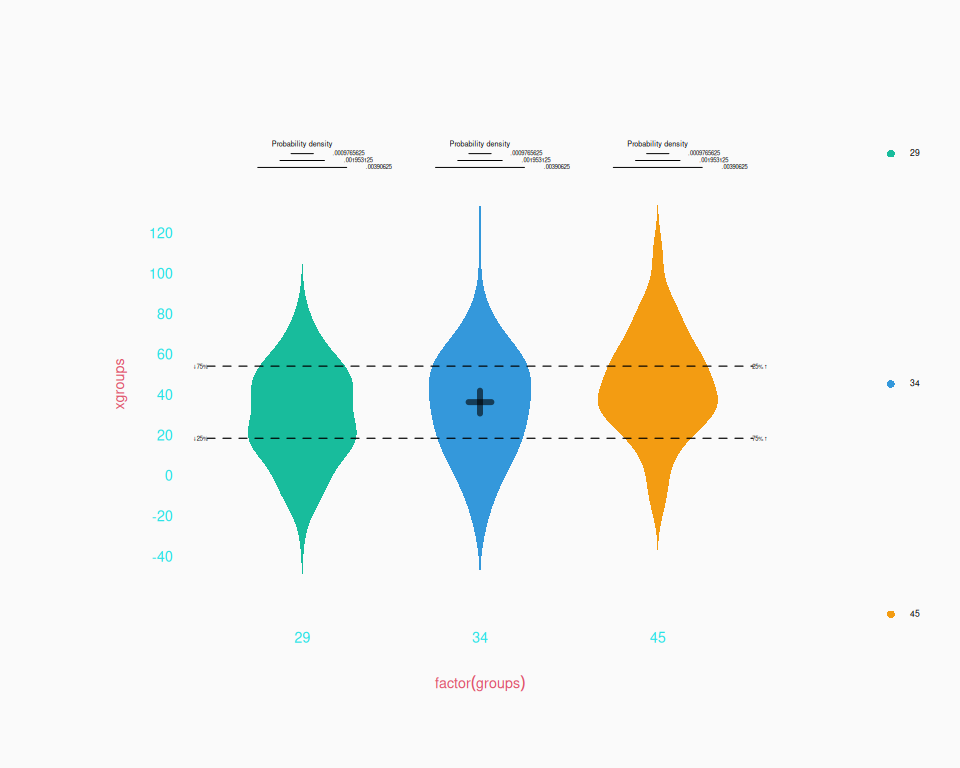
A similar, more intuitive alternative to the box plot is the violin plot, named for its typical shape:

Three (or more) Dimensions

Sometimes we’d like to visualize the relationship between more than two variables. This is really only necessary to visualize interactions between variables. If there is no interaction to visualize, you might as well visualize each pair of variables separately.

Numeric X Categorical X Categorical

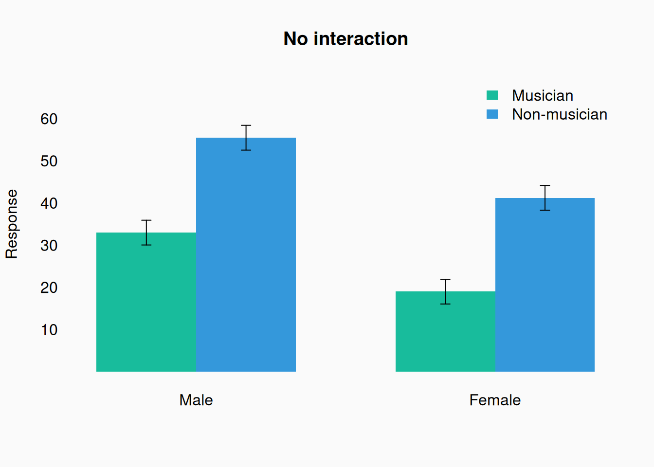
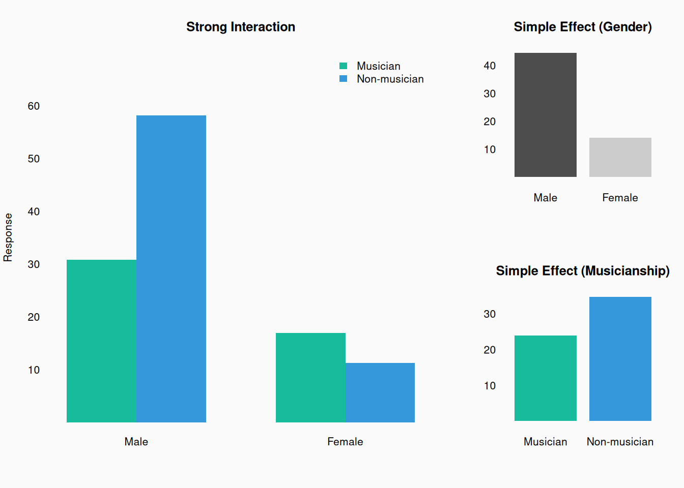
A common case is one numeric variable (usually the dependent variable) being predicted by two categorical variables. The standard approach is the calculate the mean of the numeric variable for each combination of the categorical variables, and to plot these means, perhaps as bar plots:

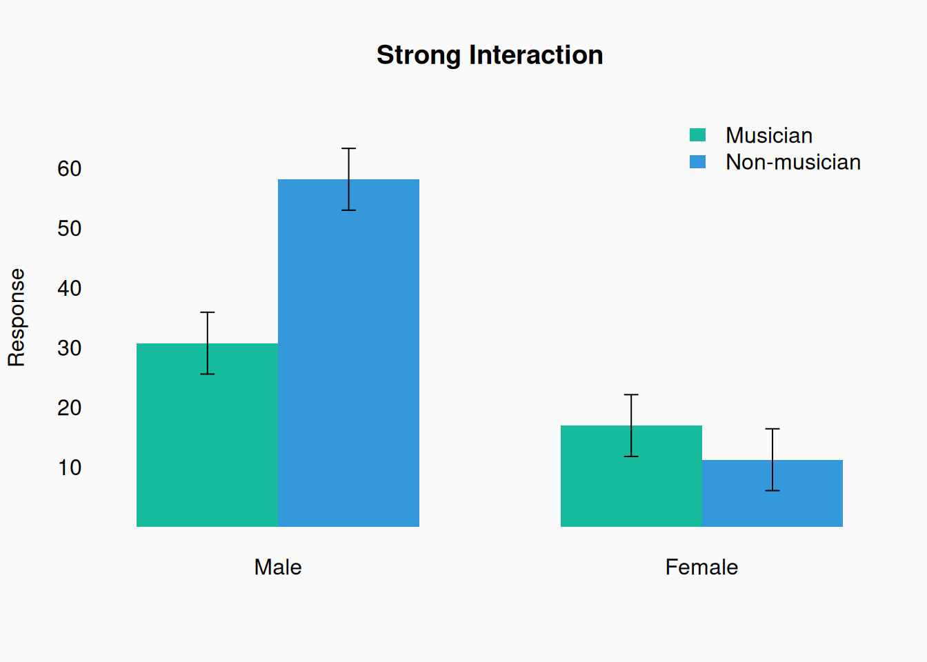
Remember, these plots can only really show the mean, not the shape of the distribution. If there is an interaction, the relative size of of the bars should be different in the two groups:

This example illustrates the importance of 3-dimensional visualization to see interactions. If we look at only the main (isolated) effects of gender and musicianship, we don’t see how they interact.

Categorical X Numeric X Numeric

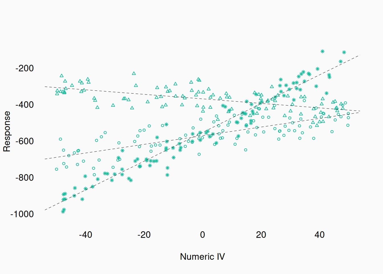
When numeric (integer/ratio) data gets involved, plotting more than two variables becomes increasingly difficult. Generally, showing multiple dimensions through more plots is the best approach. You can also use other factors to represent a third variable—e.g., color or shape. However, these other variables are much less precise communicators compared to length/position. They work best when used to indicate a categorical variable with few levels.
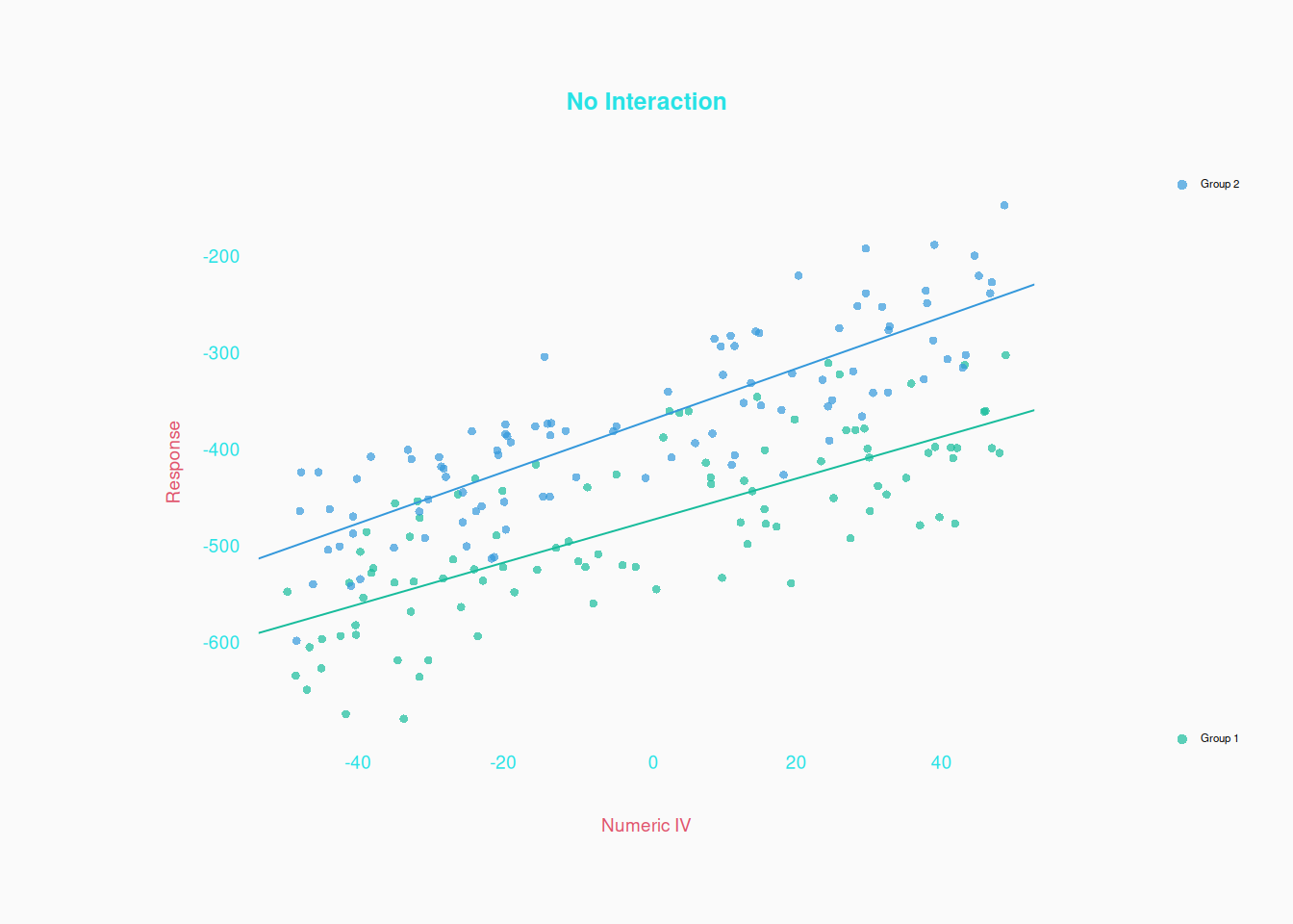
Here is a scatter plot showing the relationship between one numeric independent variable (X axis), one binary independent variable (color), and a numeric dependent variable (Y):

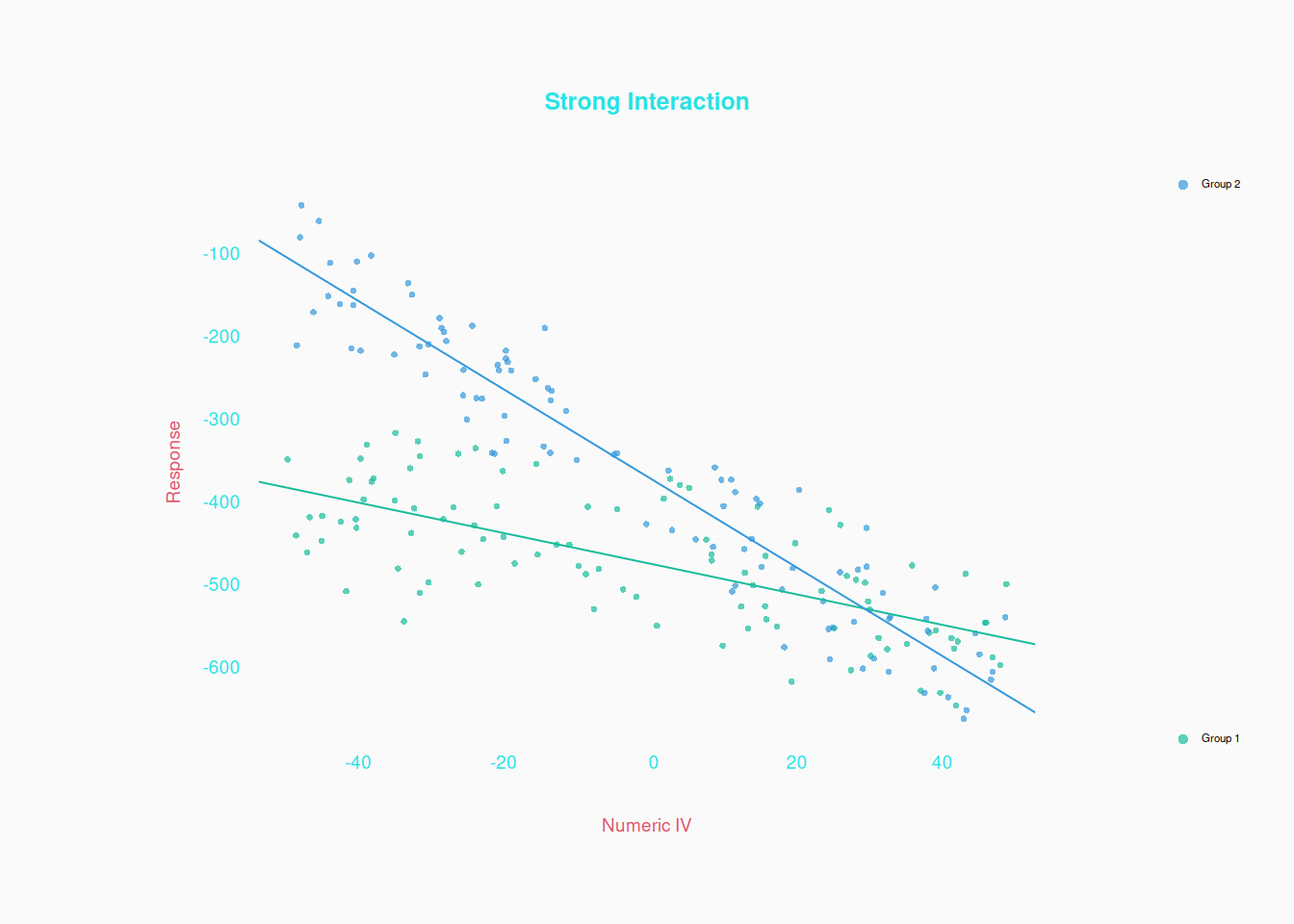
Notice that the two regression slopes (one for each group) appear to be the same. This indicates that there is no interaction between the two independent variables. If there were an interaction, we’d see different slopes in the two groups, like this:

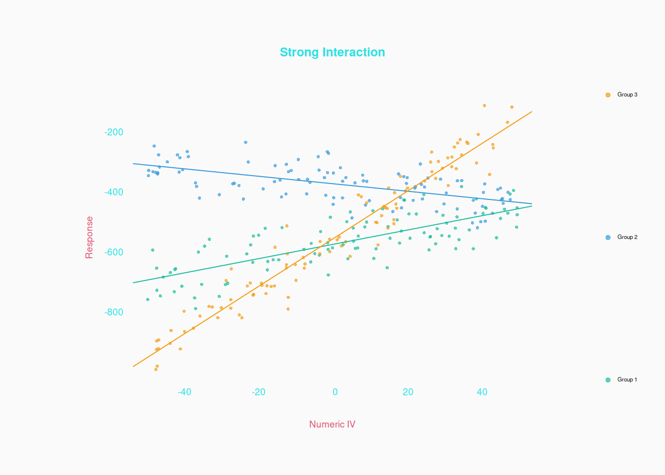
Using colors like this works fine when there are few groups. Even three is okay:

But if there are too many groups (colors) it becomes unreadable!


Some people prefer using symbols to colors, but I wouldn’t recommend it:

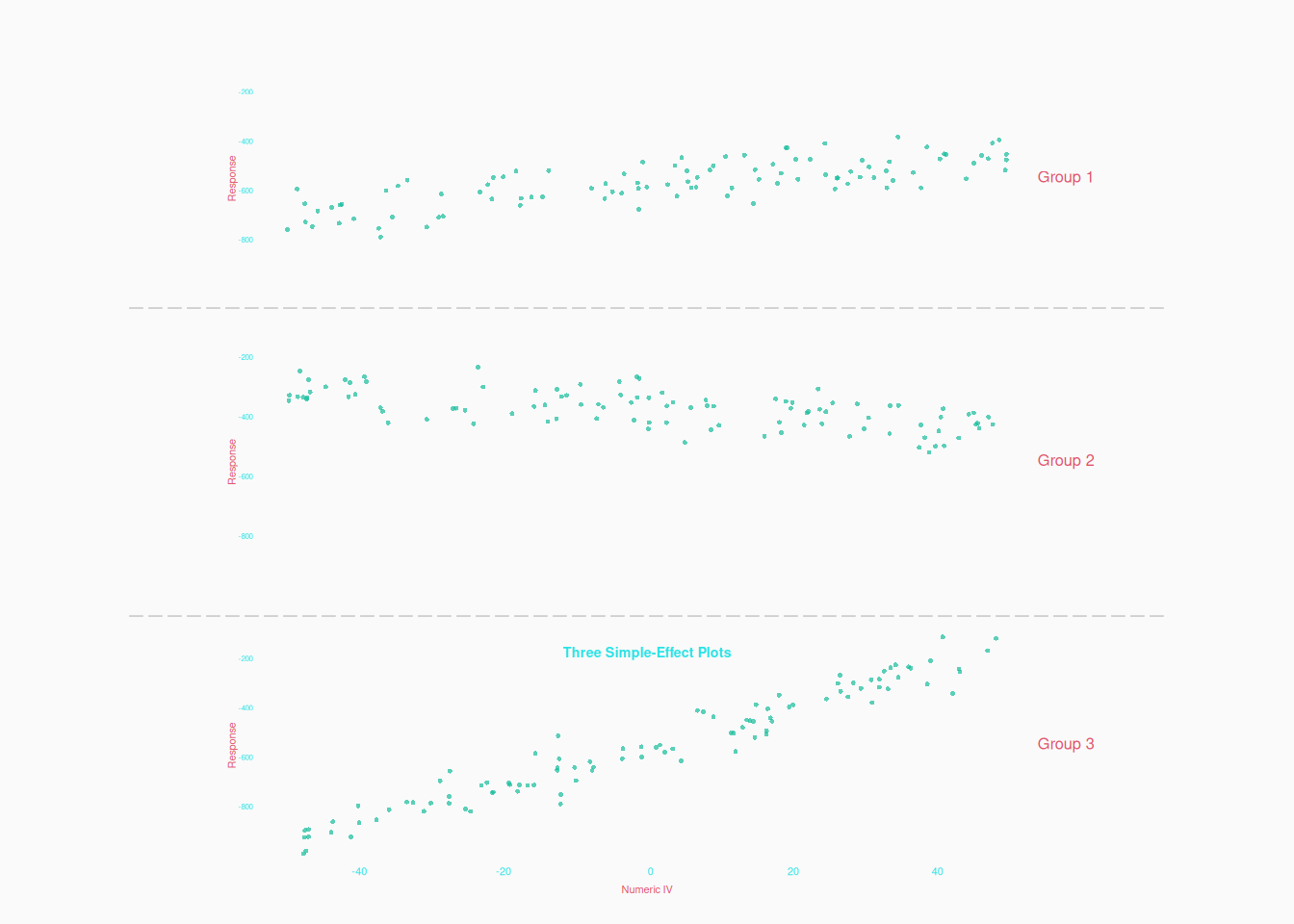
A final option, which might be the best option in many cases, is just three (or more if necessary) separate scatter plots. Even though each plot shows only a simple effect, we can see the interaction by comparing the plots:

Numeric X Numeric X Numeric

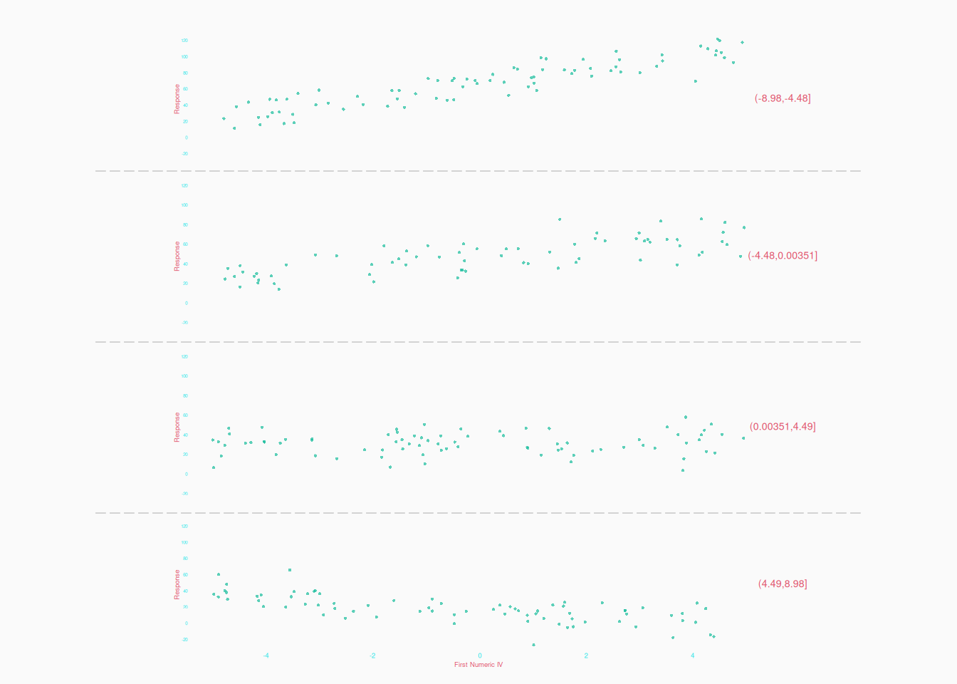
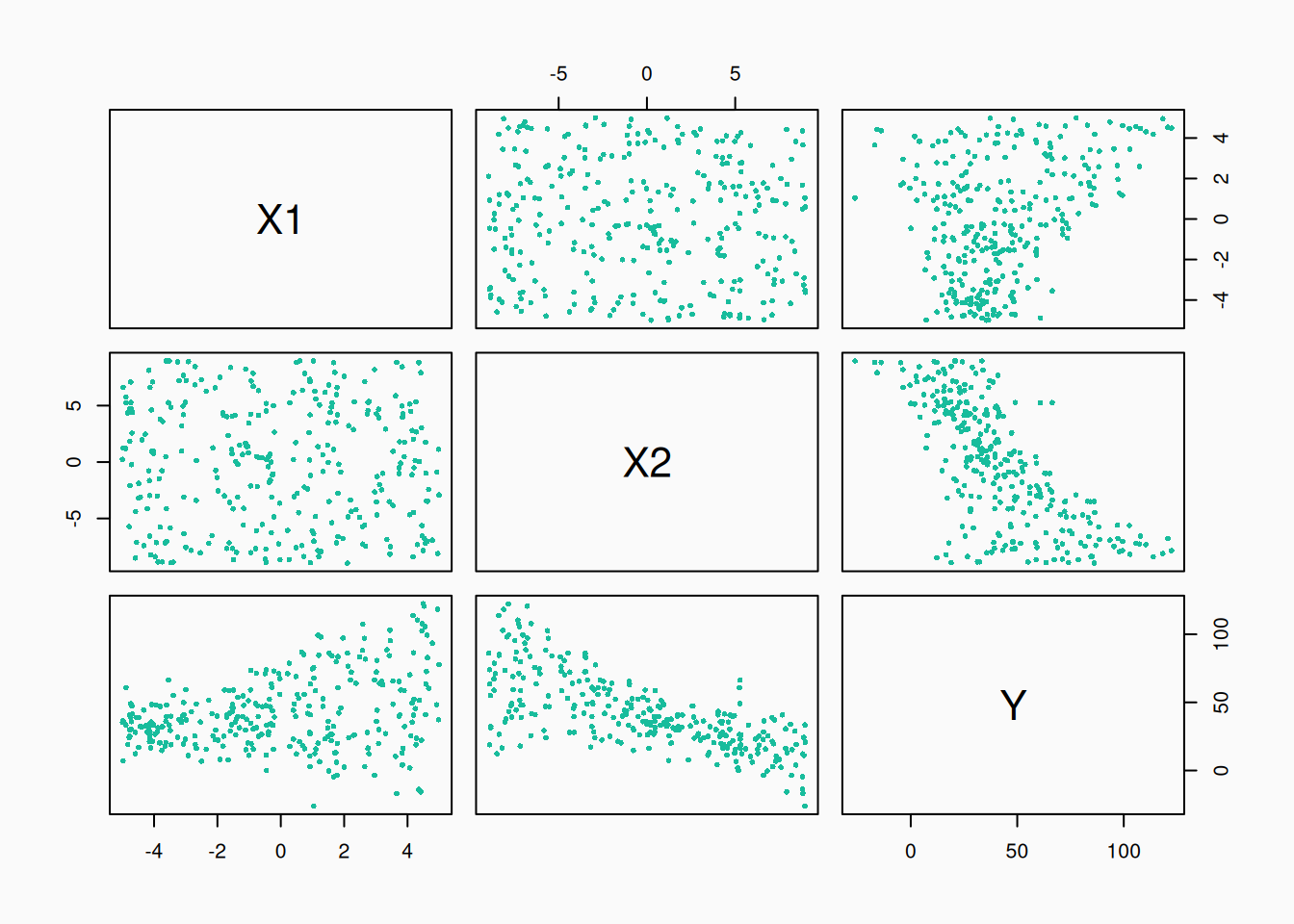
What about multiple numeric independent variables? The simplest, easiest to parse, approach is to make multiple plots, one for each pair of variables.

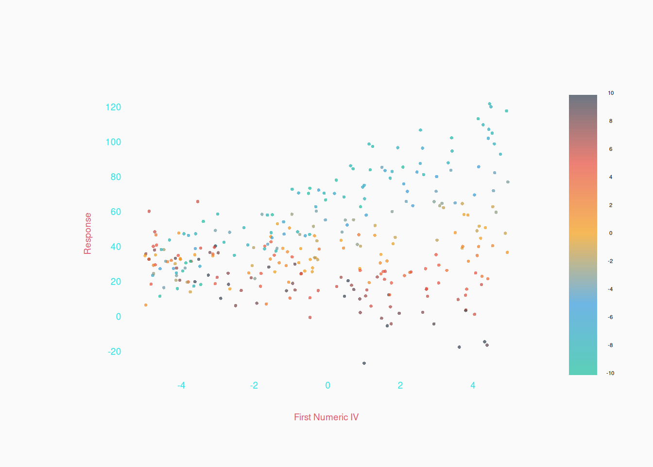
But we can’t really see if X1 and X2 interact. We could try using a range of colors to represent X2.

But it’s probably better to do multiple plots, dividing the second IV into ranges:


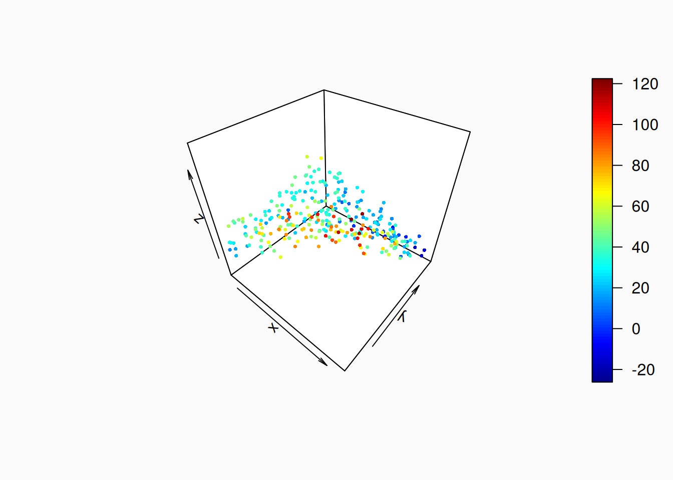
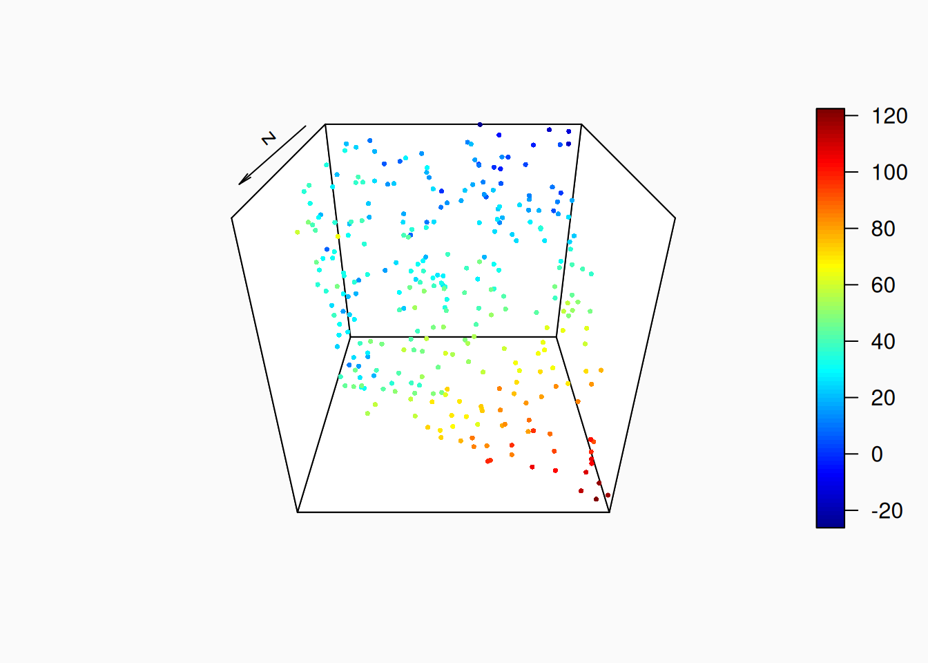
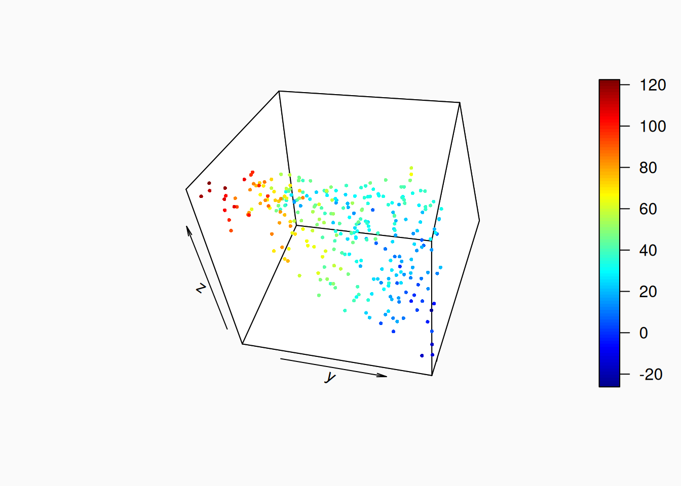
Don’t do 3d plots! 3d plots are garbage. Or at least, its very hard for them to not be garbage. Why? Because they depend hugely on what angle you look at the 3d space from. Here are three angles on the same 3d scatter plot:

Effect Size and Direction

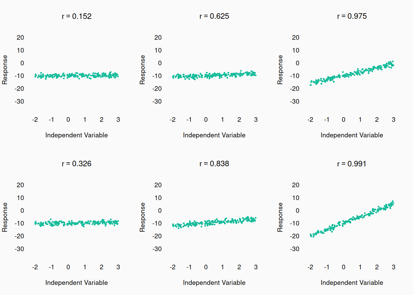
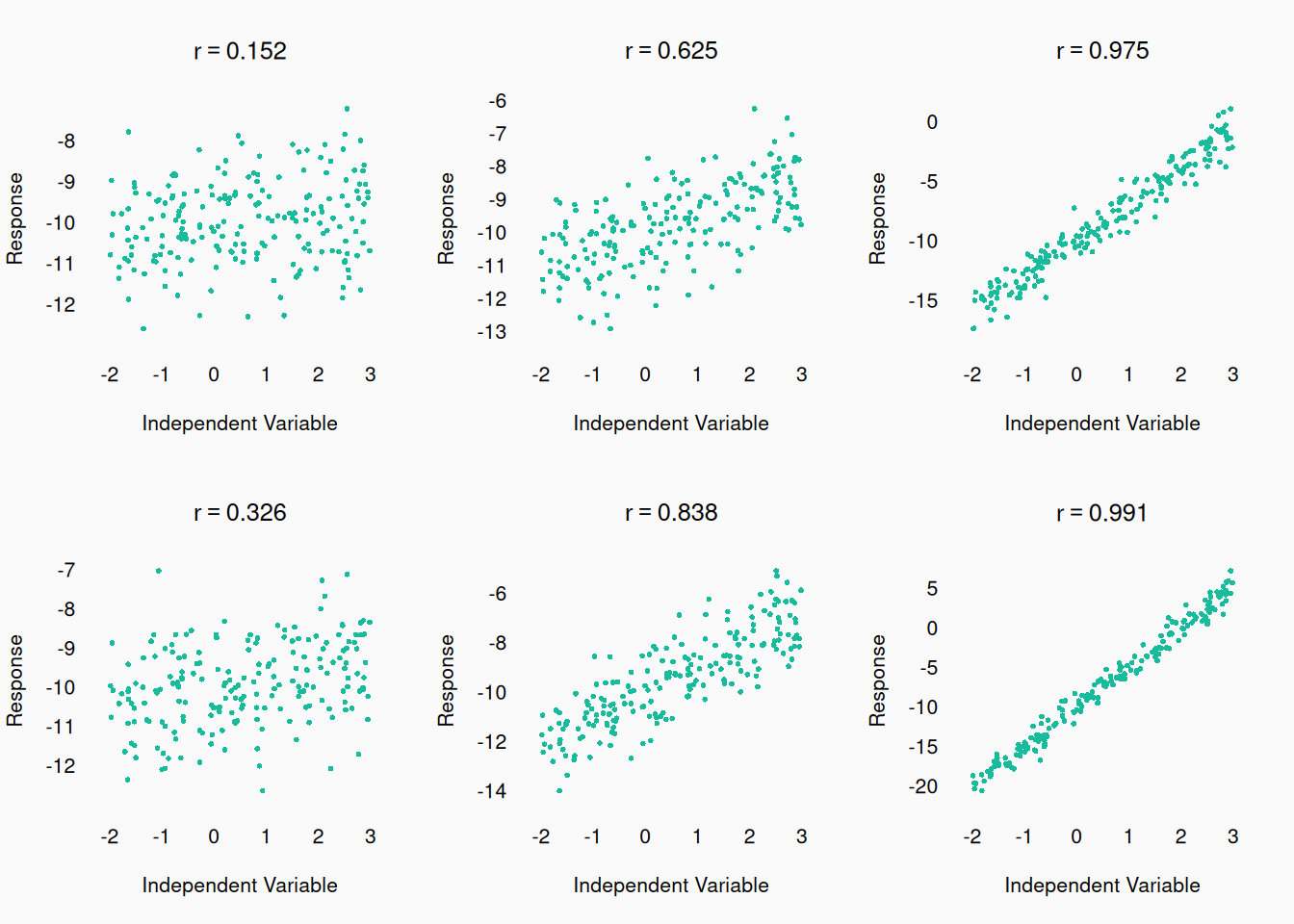
Graphs are the best place to get, and convey to your readers, effect sizes: the strength (and direction) of the relationship between variables. We will talk about specific formal ways of quantifying effect size later, but generally, visuals are the best way. Here we can see how different correlation coefficients (\(r\)) can relate to a scatter plot:

We can also look at the same correlatiosn with changing Y-axis:


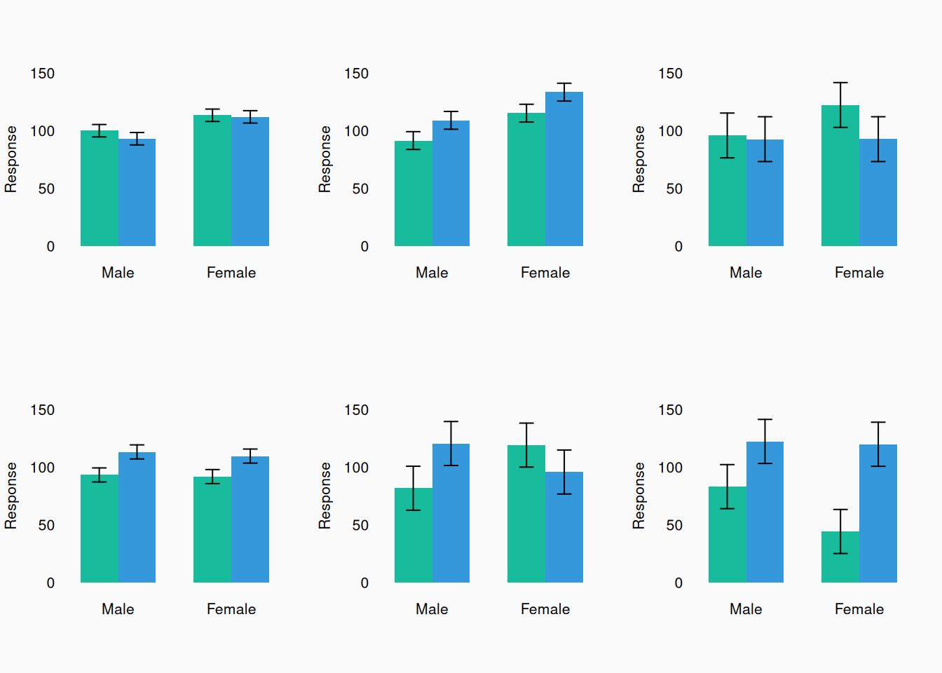
Here are some bar plots with varying effect sizes:

A story

In grad school, one of my fellow students (not Dr. Arthur!) was preparing to present some work at the International Society for Music Perception and Cognition (ICMPC) conference, in Korea in 2014. They did statistical tests on their data and the null hypothesis didn’t seem to be consistent with the statistics, so they were ready to conclude that their data supported their hypothesis. However, the morning before presenting, they graphed their data and saw that the effect (a linear correlation) they were testing was actually going in the opposite direction to what they predicted! They predicted a positive effect/slope but there was a negative slope! They had to rewrite their entire presentation before they could present. If they had visualized their data early on, they wouldn’t have been in this position.

Best practices

Let’s talk best practices. Good data visualizations should:

  • Avoid distorting data.
  • Don’t hide information.
    • Show the complete distribution of data if you can.
    • “Reveal the data at several levels of detail, from a broad overview to the fine structure” (Tufte 2001, 13).
  • Minimize “ink” (ibid).
  • Be consistent:
    • Use colors consistently throughout a paper.
    • Use consistent text sizes and fonts.
    • Use consistent X and Y axes.
  • Serve a clear rhetorical purpose in your paper.
  • “Be closely integrated with the statistical and verbal descriptions of a data set” (ibid).
  • “Encourage the eye to compare different pieces of data” (ibid).

We can only cover so much here: I highly recommend that you read Edward Tufte’s (2001) hugely influential book on data visualization: The Visual Display of Quantitative Information.

Axes

In every graph, both axes should always be labeled and include a scale. And make sure that the axis labels are actually big enough to read!

Each axis range should always show (at least) the full range of data observations. However, for variables with fixed theoretical ranges, you should generally show the full theoretical range, even if your data doesn’t cover the whole range. For example, proportions go from 0 to 1, so you should generally show this whole range. If participants are responding given a response scale of 1–9, show the full range from 1–9, even if their responses never got higher than 7.


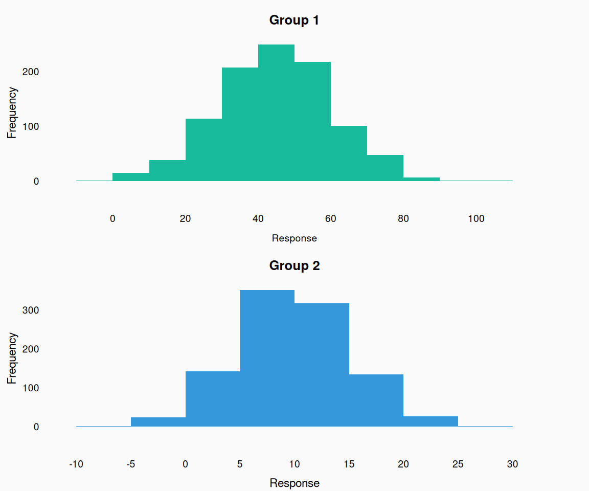
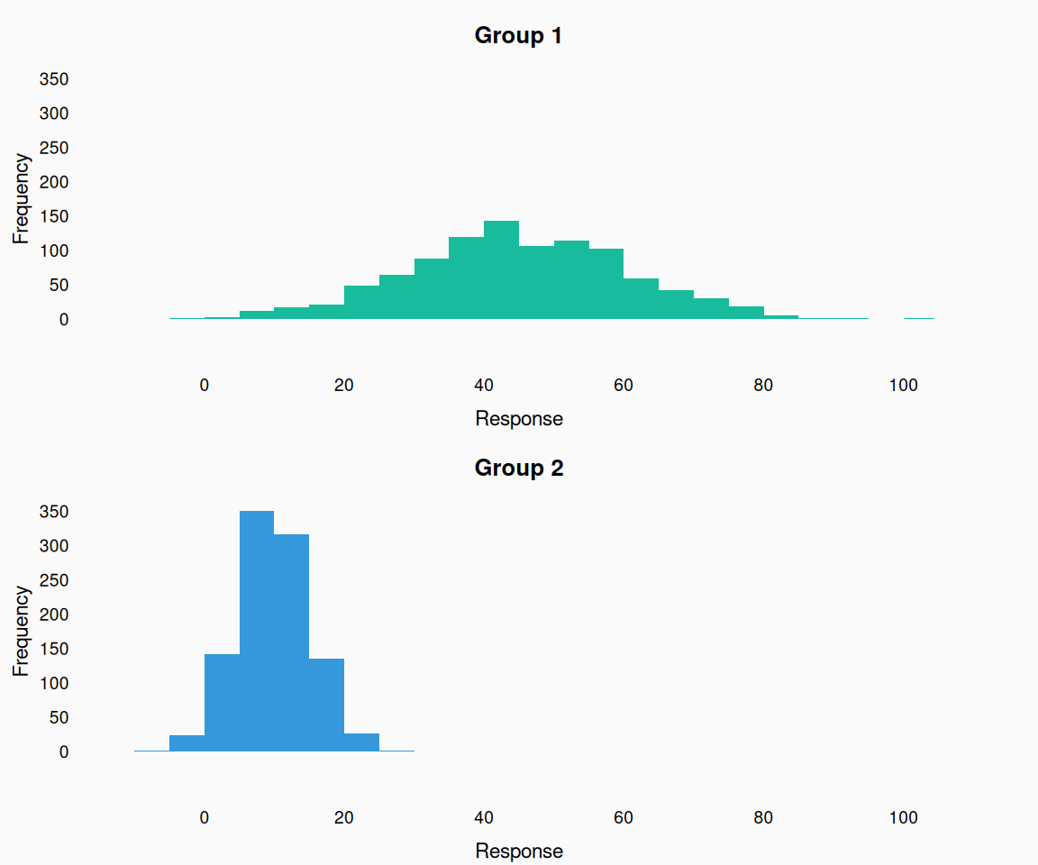
When plotting the same variable multiple plots, use the same range each time.

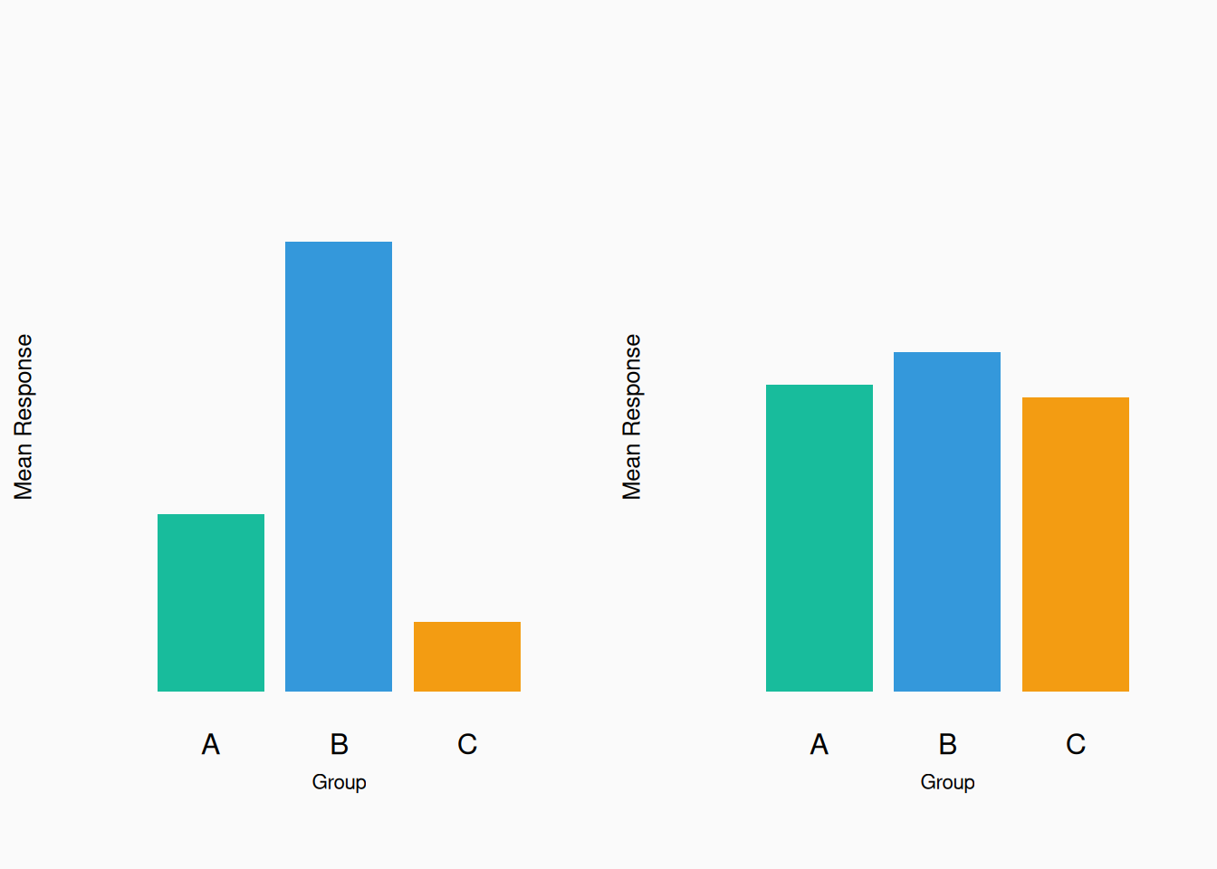
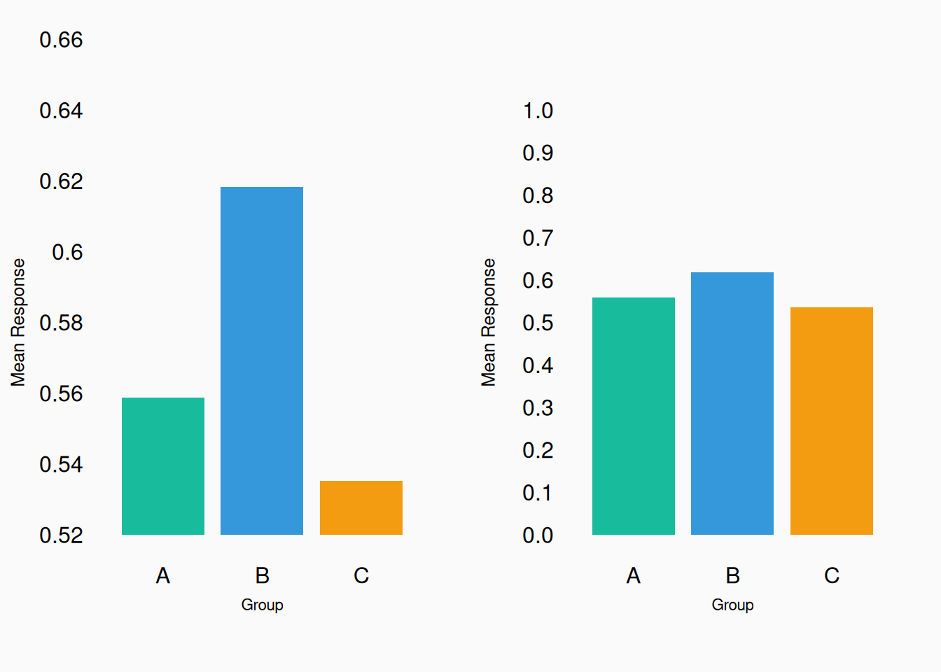
Very different results right? Well…

They are actually the same data! The left plot exaggerates the effect size—don’t do this! Show shared axes consistently across plots:

Bad!

Good! Now we can see how the two variables differ.


Bad!

Good!

Area vs Height

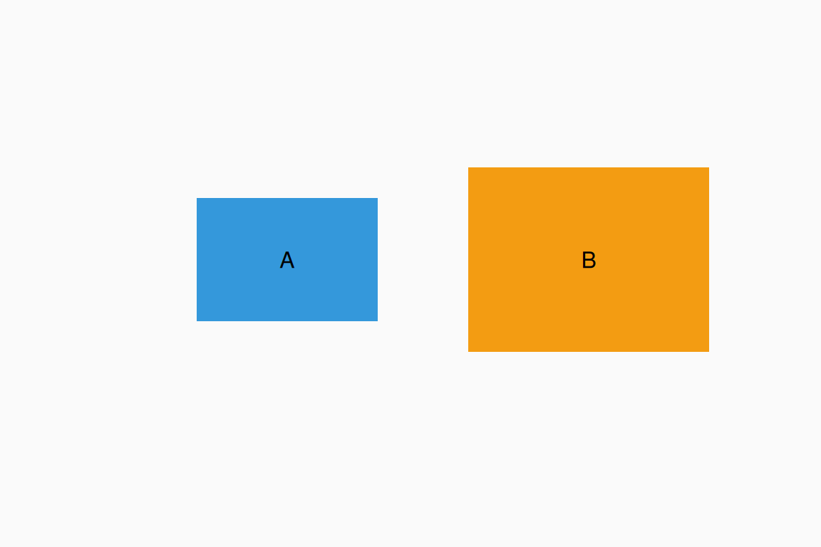
When comparing the size of two shapes, humans tend to (intuitively) respond to the relative area. However, we aren’t good at doing this precisely. How much bigger is B than A?

B is twice the size (area) of A. This is why pie charts are often criticised.

Show everything

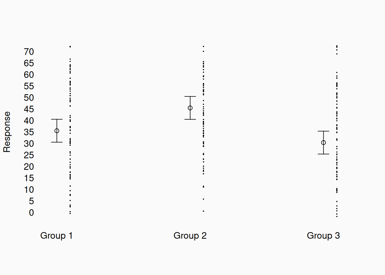
We often “just” plot means.

But we are missing lots of information here. Show me all the data!

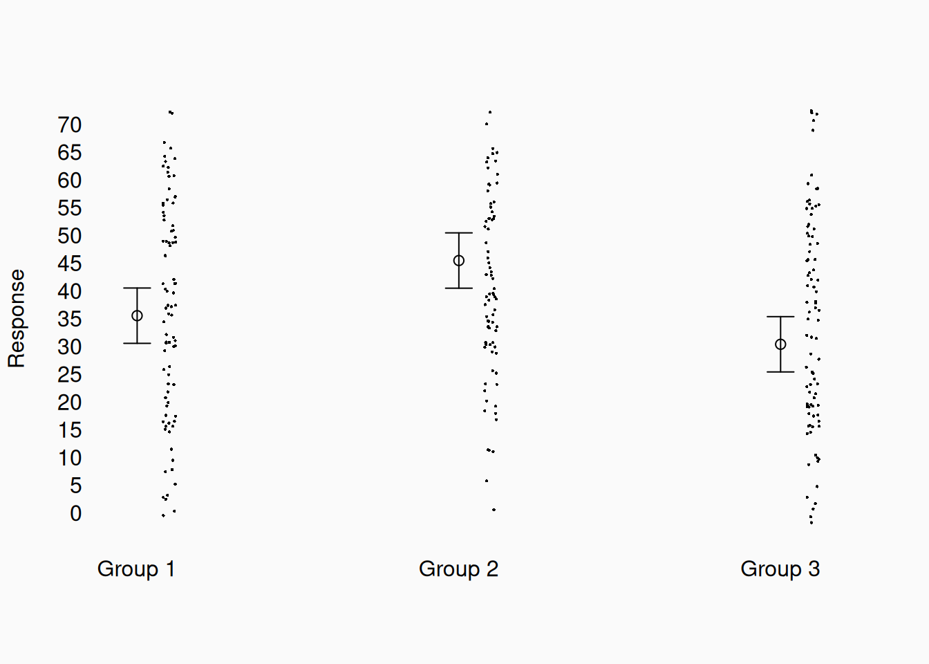
Now we can see not only the mean, but also the distribution of the data in each group, and that the data is much more variable than the first plot suggested. It can be useful to apply random “jitter” to the x-coordinate of the points, so they aren’t on top of each other:


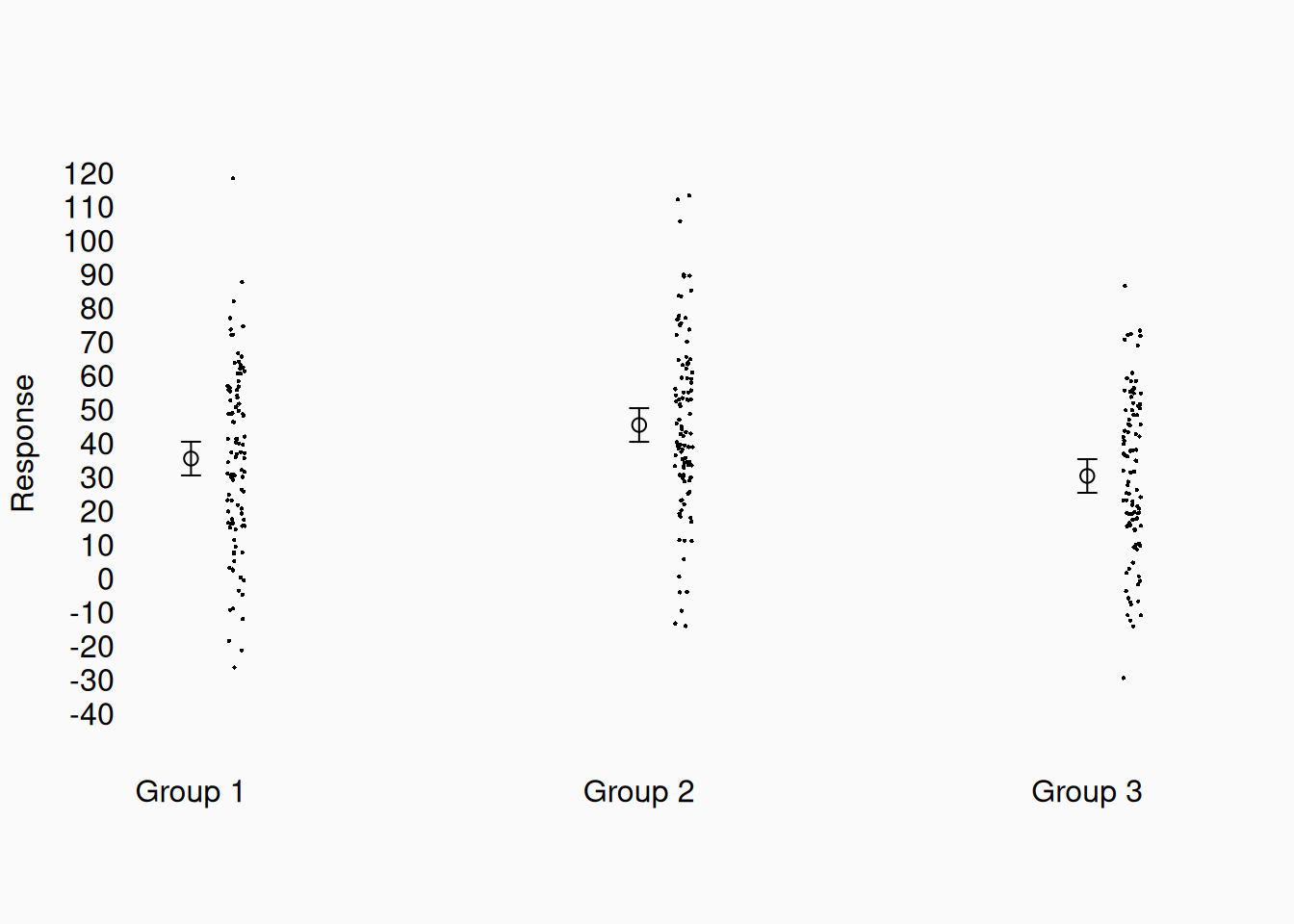
When showing all the data, make sure to show the whole range. In the previous graph, I used the Y-range that showed the three means in one screen. However, now that we see all the data, there are actually data points off the screen, which is misleading. Let’s show the full range of data points:

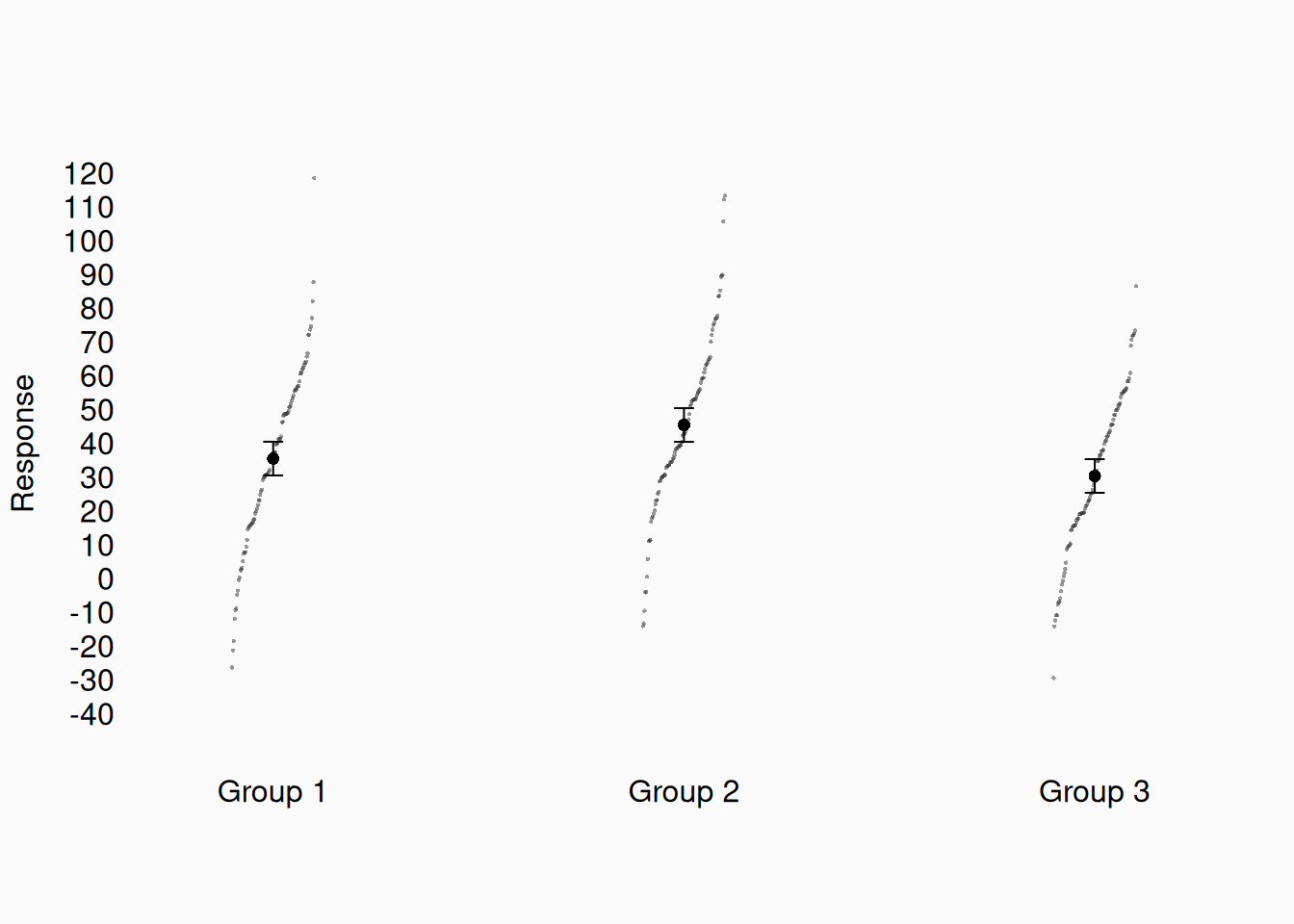
This is much better, because we get a much more realistic impression of the amount of noise in the data! We make this even better by sorting them to get quantiles!


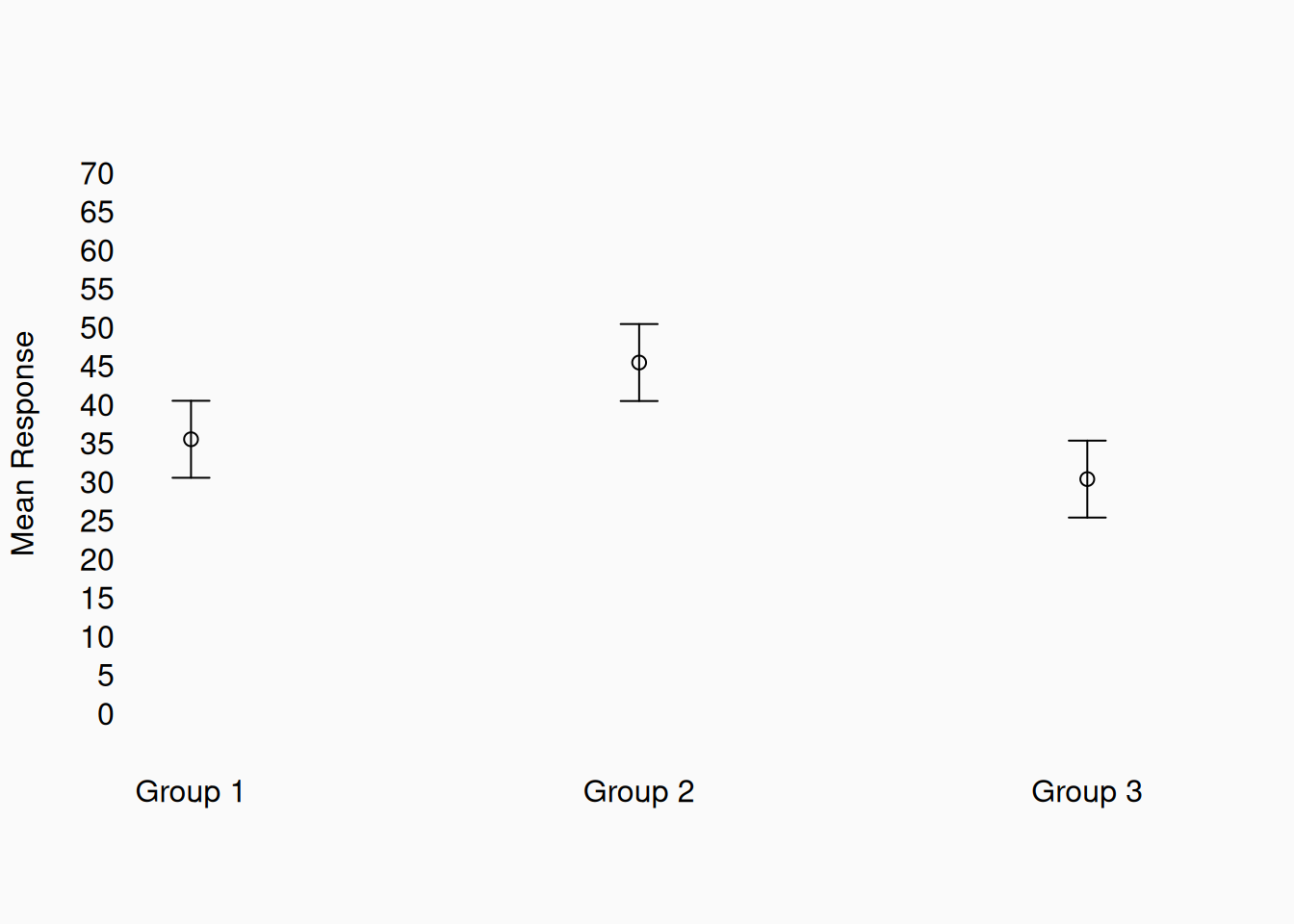
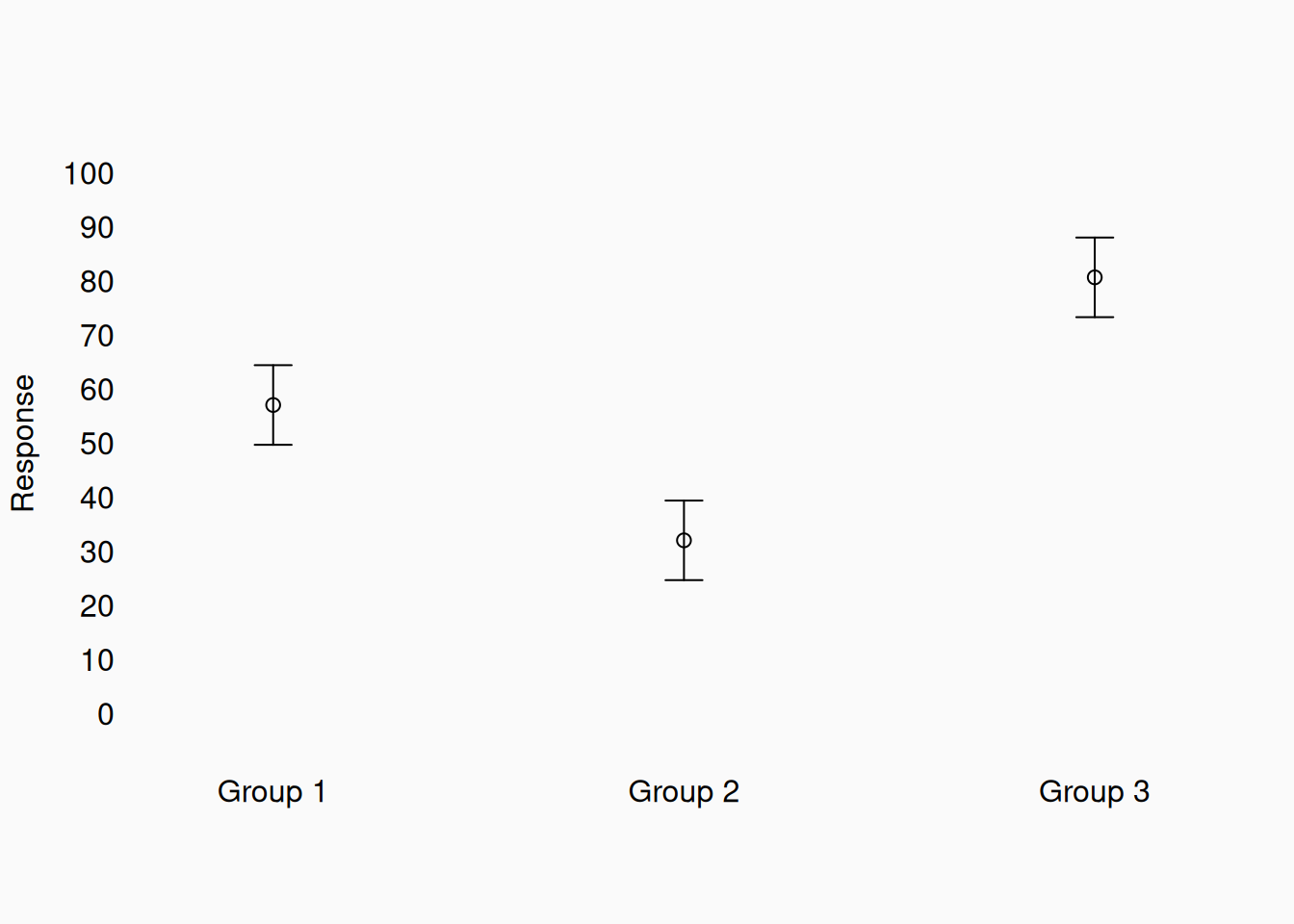
Do we really need to do this? Yes! Many papers show really misleading graphs. You don’t want to mislead yourself or your readers. Check out this plot of data, which you might see in a paper:

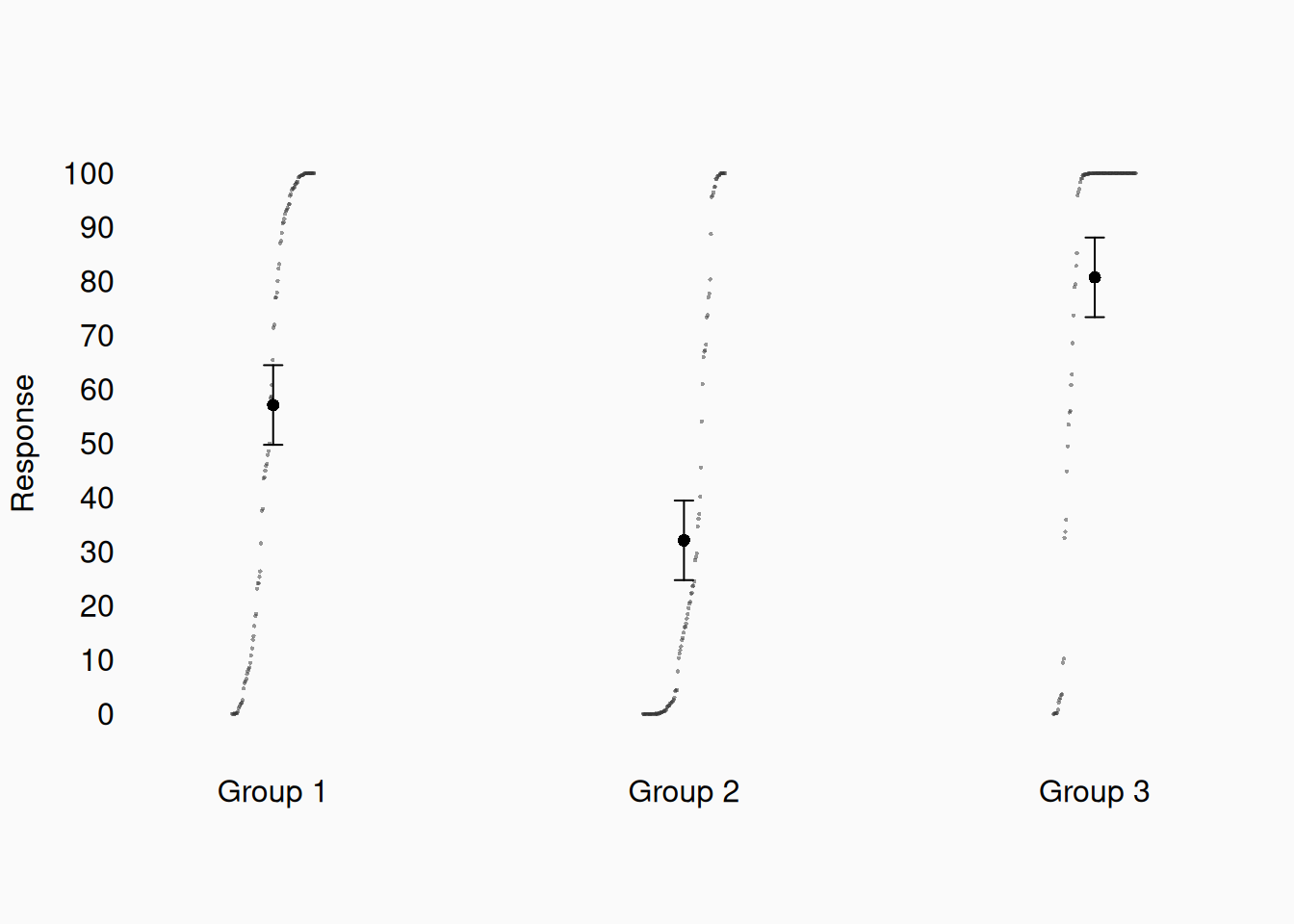
Three groups of data, with some confidence limits. It seems like group 2 is less than the other two, etc. Let’s look at all the data, as I suggest:

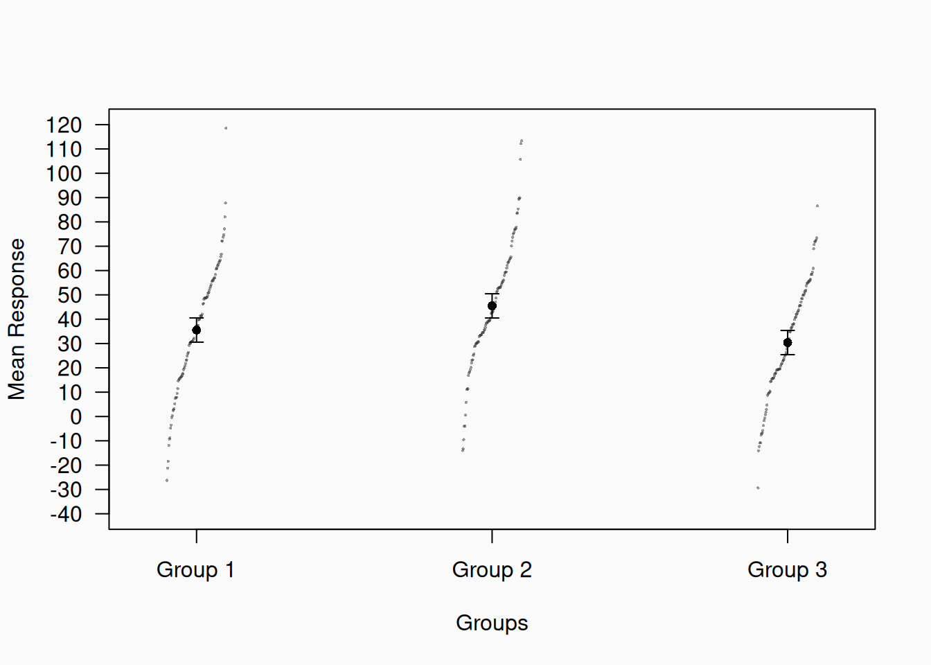
What can we see now? The (small) effect size is more evident, as we can see how much actual variability there is in the data. We also can see that there are strong ceiling and floor effects, with responses bunching up at bounds (0 and 100). Group 3 users apparently wanted to go past 100, but weren’t able to. We can’t see these problems unless we look at all the data.

Minimize ink

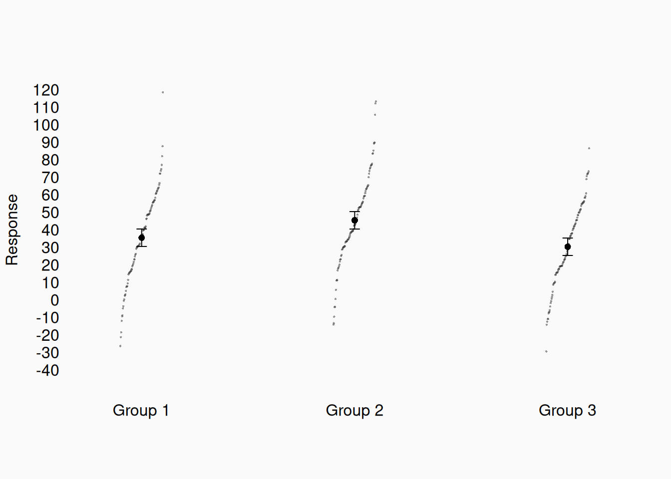
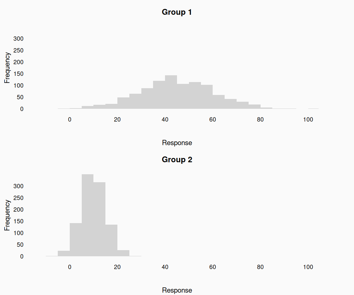
Don’t draw anything that doesn’t serve a purpose! Many plots have lots of unnecessary “ink” on them (Tufte 2001)—strip that away to make cleaner, beautiful plots.

Garbage!

Better!


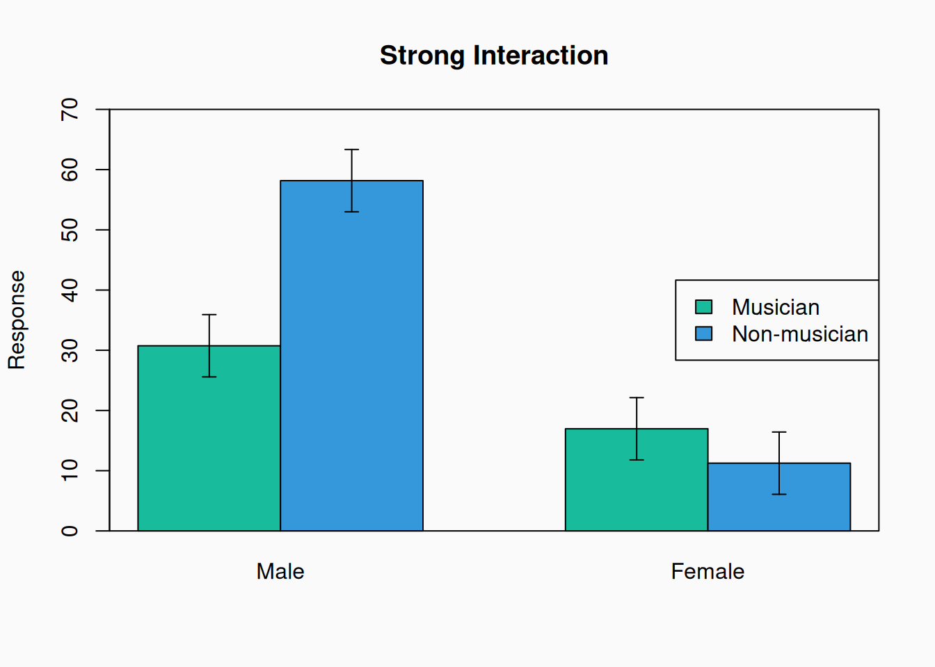
This is bad:

What purpose do the bounding box and tick marks serve? None; Get rid of them. The “Groups” label is also redundant, so drop that too:


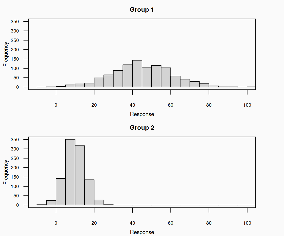
This is bad:

This is better:


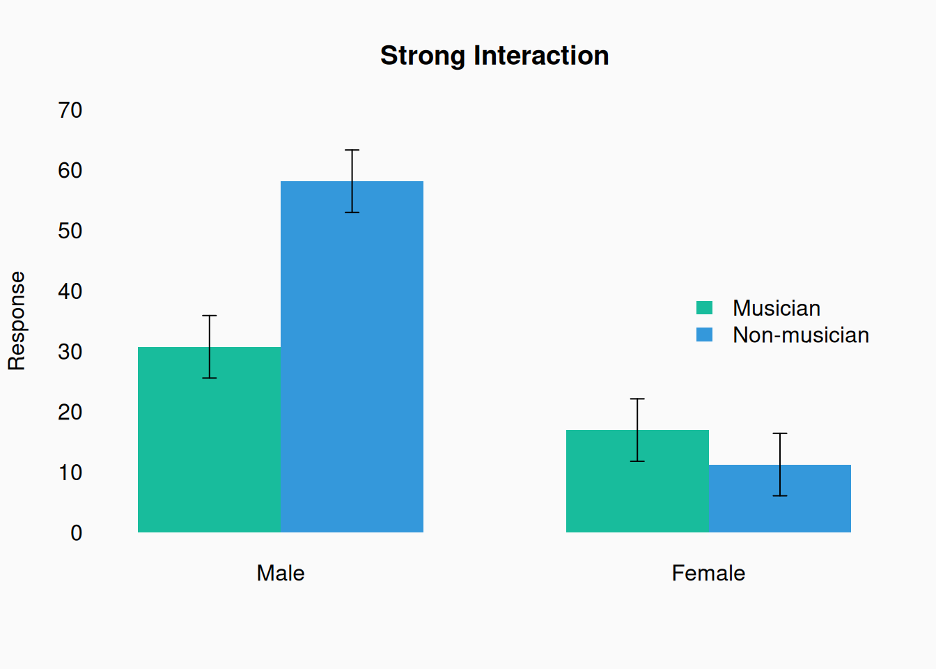
This is bad:

Why do we need so many borders on everything? (On the bars, on the legend, on the boxes in the legend…) This is better:


Defaults

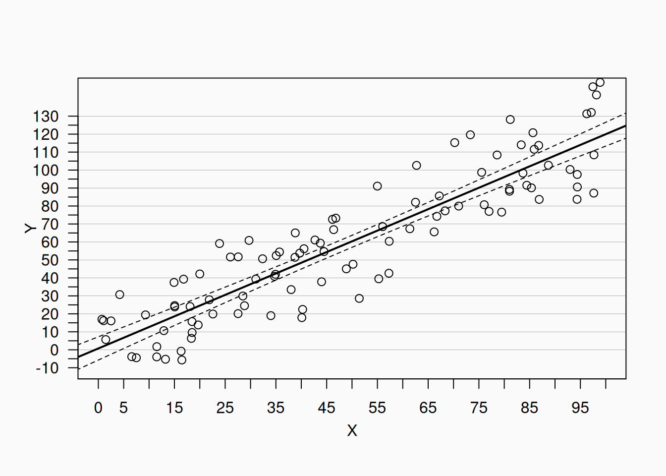
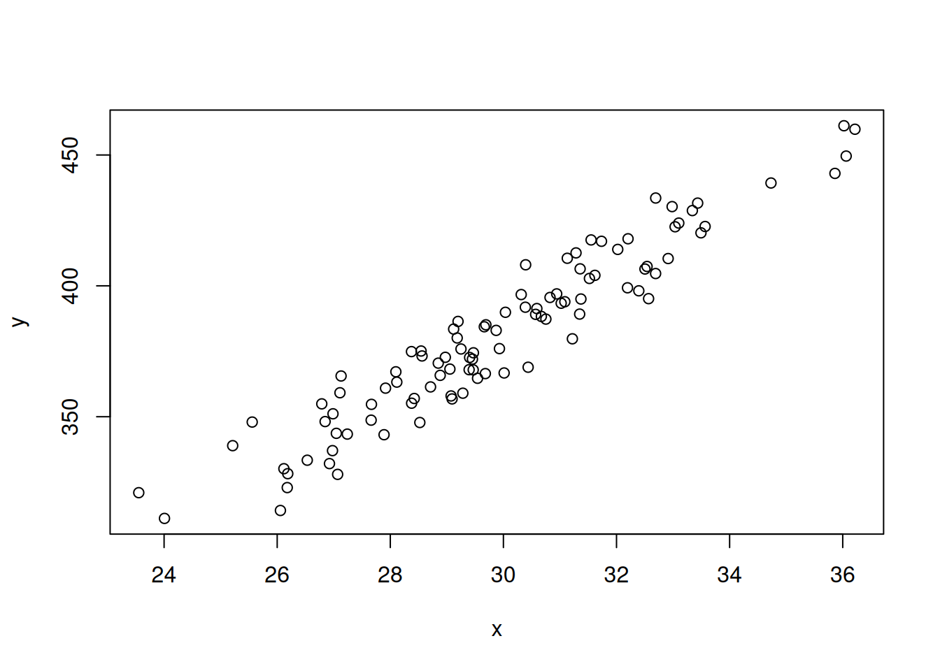
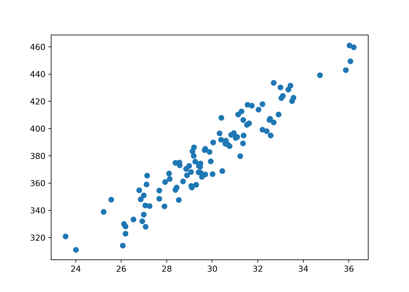
Don’t trust your graphical software’s default styles! They always include unnecessary cruft. For example, here is R’s (base) default scatter plot style:

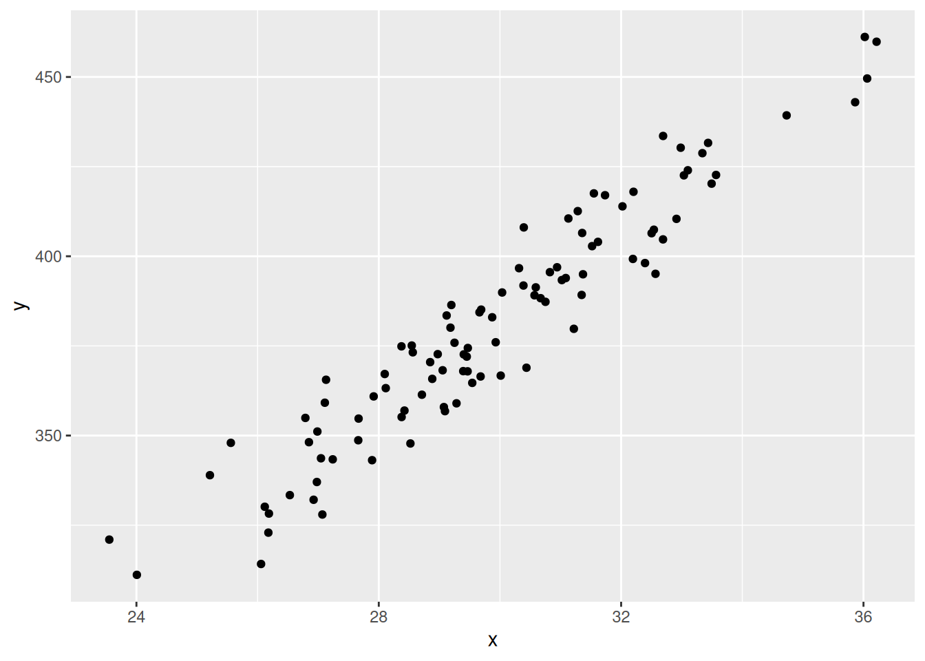
And GGplot’s (R):

Matplotlib’s (Python):

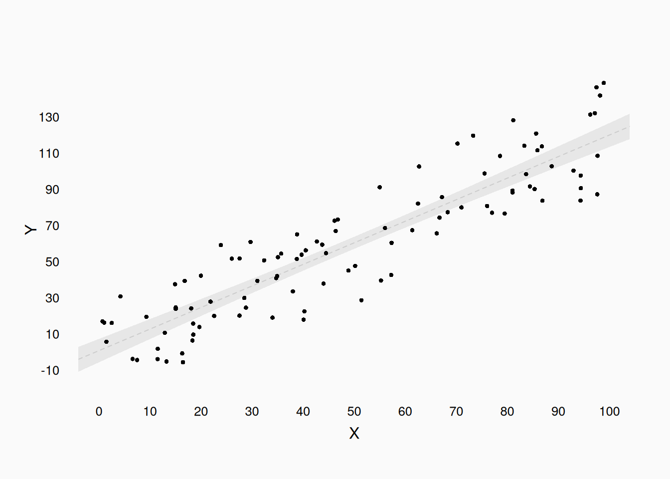
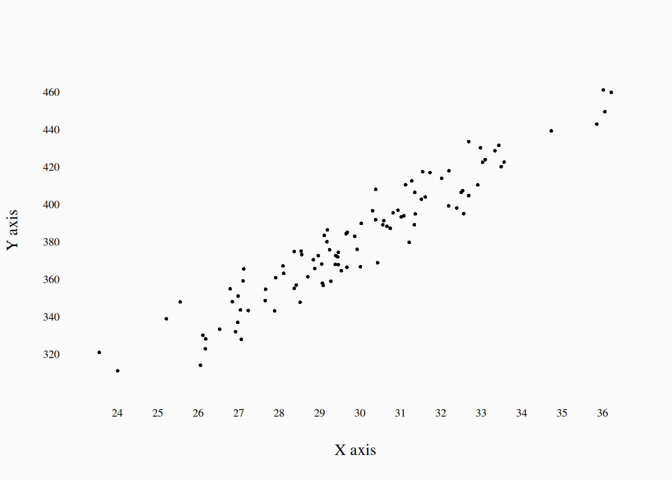
Here is a much better plot:

Mantras

Spot-check thrice, then check again

Data has problems; Always. Look at (or listen to) the data closely. Search out errors, by exploring random subsets of the data as well as any obvious outliers. Is the data formatted correctly? Is anything missing?

Draw your conclusions

Visualizing your analysis is essential to understanding your results and conveying that understanding to your audience (“graph it to grasp it”). Visualizing is an important part of data spot-checking (“plot it to spot it”). Visuals are also one of the best ways of judging and conveying effect size: does the effect look meaningful when you put it into a meaningful graph? (“See it to believe it.”)