49 Goodness-of-Fit

(Modified on 2026-08-12)
3,111 words

In previous readings we discussed the basic idea of inferential statistics: We compute “statistics” from a sample (the data we actually have) and use them to make inferences about the population—all the data that “really” exists. In order to make inferences, we typically make certain assumptions about the population of data and about our sample; for example, we might assume that the population is normally distributed and that data points in our sample are independent.

We can calculate what the distribution of sample statistics would look like if we were to take a huge (infinite) number of samples.

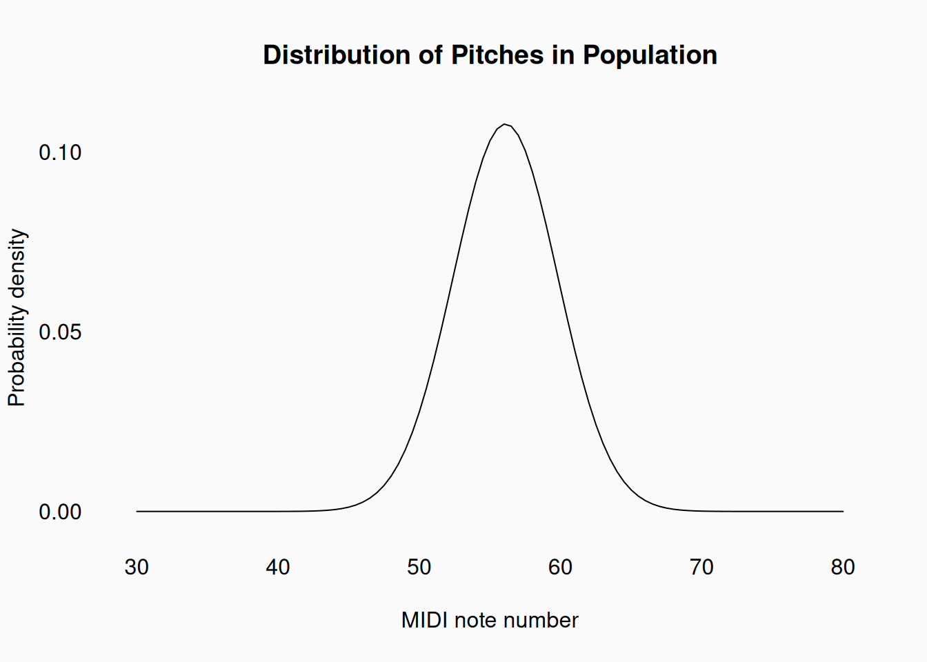
Given such assumptions, we can calculate what the distribution of sample statistics would look like if we were to take a huge (infinite) number of samples. For example, consider the absolute pitch height (in MIDI numbers) of vocals in commercially-released popular music: the population of all pitches sung in all Western commercial releases. (There are a lot of different operational definitions needed here, but we won’t worry about that right now.) Imagine that we somehow magically knew that this population follows a normal distribution with a mean $\mu =56.1$ and a variance of $\sigma^2 =13.69$, like this:

If we sample from this population and calculate the sample mean ($\bar{x}$), the sample mean will never be exactly 56.1; $\mu \neq \bar{x}$. However, it will probably be close. But how close? We can’t know for sure. But imagine if we did this many times—that is, we collected many independent samples of pitches from the population and calculated the mean of each sample. We could inspect all these many sample means and see how spread out they are, giving us a rough estimate of “how close” any one sample mean $\bar{x}$ is likely to be to the population mean $\mu$.

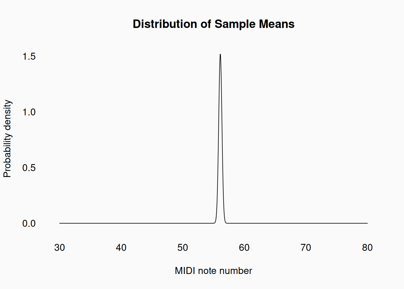
Of course, we don’t typically have the resources to take a whole bunch of samples of data. Fortunately, thanks to some fundamental statistical theorems, we don’t have to. In fact, the central limit theorem tells us that, if we were to sample an infinite number of times—calculating the mean of each sample—the sample means will actually follow a normal distribution, centered on the population mean, with a variance which is simply the population variance ($\sigma^2$) divided by the sample size $N$!

Let’s walk through this using our concrete example, where we know that the population has $\mu =56.1$ and $\sigma = 3.7$. Let’s say we decide to take samples of size $N = 200$. If we were to take such samples over and over, an infinite number of times, the central limit theorem tells us that the distribution of sample means will be normally distributed with a mean $\mu =56.1$ and variance $\frac{\sigma^2}{N} = \frac{13.69}{200} = 0.06845$. The standard deviation of this distribution is, of course, simply the square root of this variance: $\frac{\sigma}{\sqrt{N}} = \frac{3.7}{14.142} = 0.26163$. By convention, this standard deviation is called the standard error. So the sampling distribution of the mean would look like:

This all may be well and good, but you probably have (at least) two concerns: 1) we only ever get to look at one sample, so how does this “sampling distribution” help us?; 2) how do we know our assumptions about the population make any sense?

The description of the population is always theoretical; It is our model of the process that generated our data. The sample is always empirical. We want to know whether our model is a good explanation of the data; this often expressed as good “fit.” If the model is a good one, the data should fit the model well.

If, for example, we saw a sample of data that looked like this:

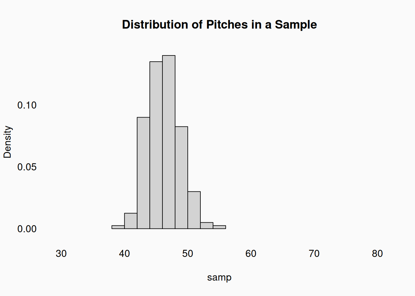
We’d think, this data is really far from what we’d expect to see if the $\mu =56.1$. Something is wrong. Maybe we are sampling from the wrong population (biased towards bass singers, evidently), or maybe we need to update our understanding of the population. Generally, we never know the “true” population mean, so we are always trying to guess (infer) what it is from data. This sample would make us revise our estimates of the population mean.

We need to judge which model “fits” the data best.

Of course, the population model I presented is clearly flawed because we know that male and female singers have different ranges. A better model of the population would incorporate a gender variable, with a separate mean for each gender. In fact, in research, we are generally interested in relationships between variables—we might also postulate that genre or release year might be variables that also affect pitch height. So our main task is figuring out which model of those relationships match reality best. To do this, we need to judge which model “fits” the data best.

We might hypothesize that gender, release-year, and genre influence pitch height in commercial recordings. The null hypothesis would be that these variables don’t affect pitch height. So what we actually want to know is does one model (our theoretical model) “fit” the data better than another (the null model).

Model Evaluation and Comparison

How do we evaluate how well a model “fits” data? How do we compare two models and judge which one “fits” better? For example, if we have a null (hypothesis) model and an alternative-hypothesis model?

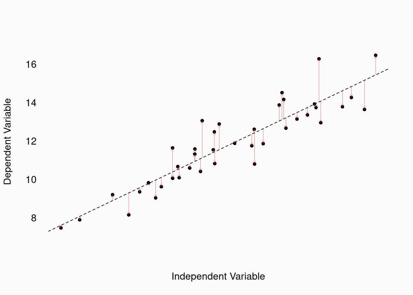
The basic idea is to evaluate how far, on average, each model’s predictions are from the actual data. We create models that can predict a specific value in the dependent (predicted) variable for every combination of independent (predictor) variables. This predicted value is usually called $\hat{y}$ (“y-hat”); The true data value is just $y$. The distance between actual data and model predictions is called residual error, or just residuals: $y_i - \hat{y}_i$

We often model a dependent variable as a linear function of a numerical independent variable—simple linear regression. Here is an example of residuals in a simple linear regression:

A different model might predict a dependent variable as a function of a binary independent variable: Here are residuals in an experiment with independent-variable groups:

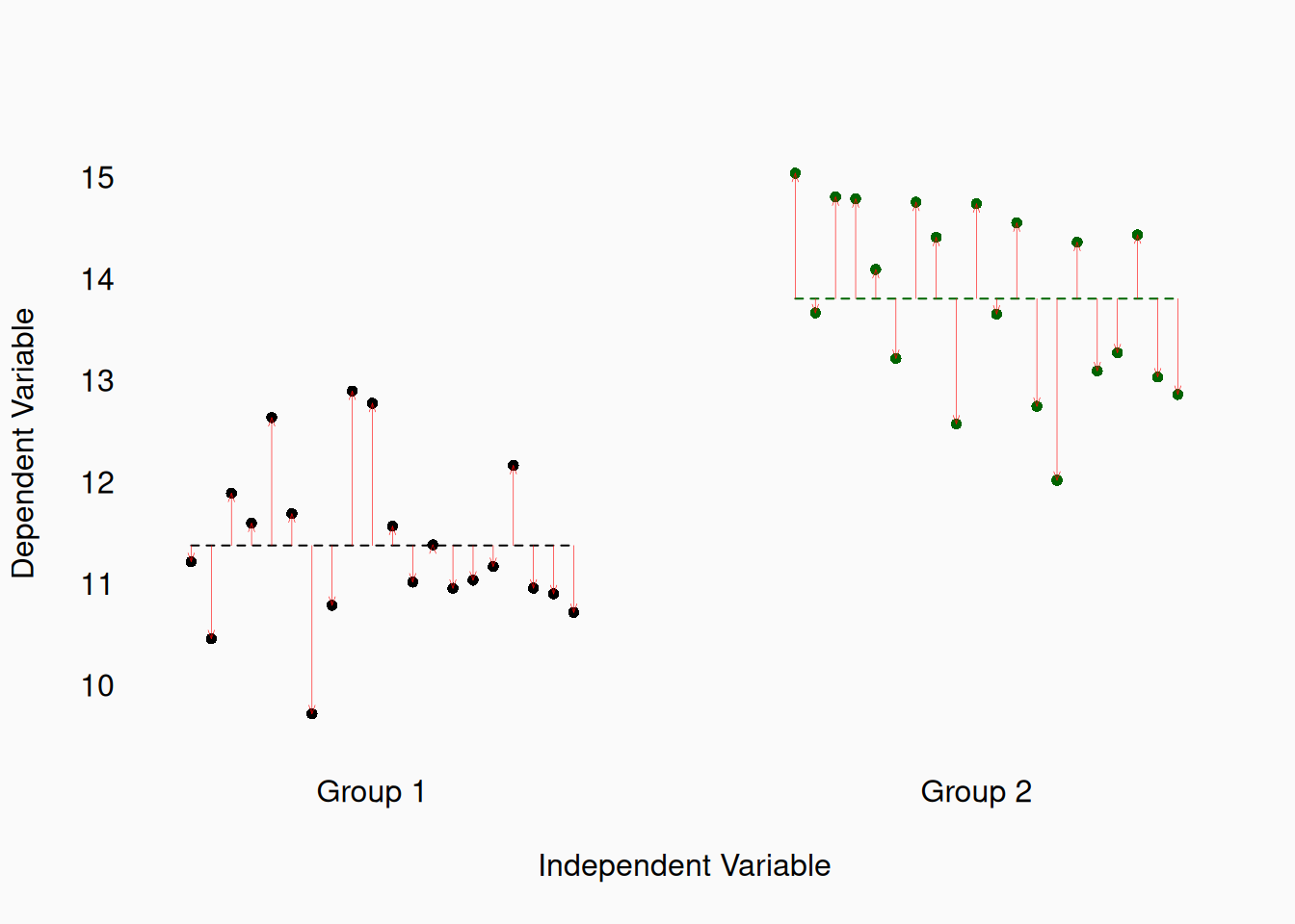
Every single data point gets its own residual. We can model the set of sample residuals—for example, by postulating that they will be normally distributed (as in the previous examples). More generally, the residuals can become the basis for an error function—a.k.a, a loss function or an objective function. An error/loss/objective function essentially summarizes the model’s residuals. We generally want to find model parameters that minimize this function (minimize residuals). This is called optimization. There are two main widely used error functions: Least Squares and Maximum Likelihood (which is equivalent to cross entropy).

Least Squares

The most fundamental error function is least squares: we seek to minimize (least) the sum of the squared residuals—the “sum of squares” (SS).

$SS = \sum_{i=1}^N (y_i - \hat{y}_i)^2$
$\min(SS) =$ least squares

Given a numeric sample, with no other information, we can find the point in the sample that minimizes the sum of squared residuals. This gif illustrates that:

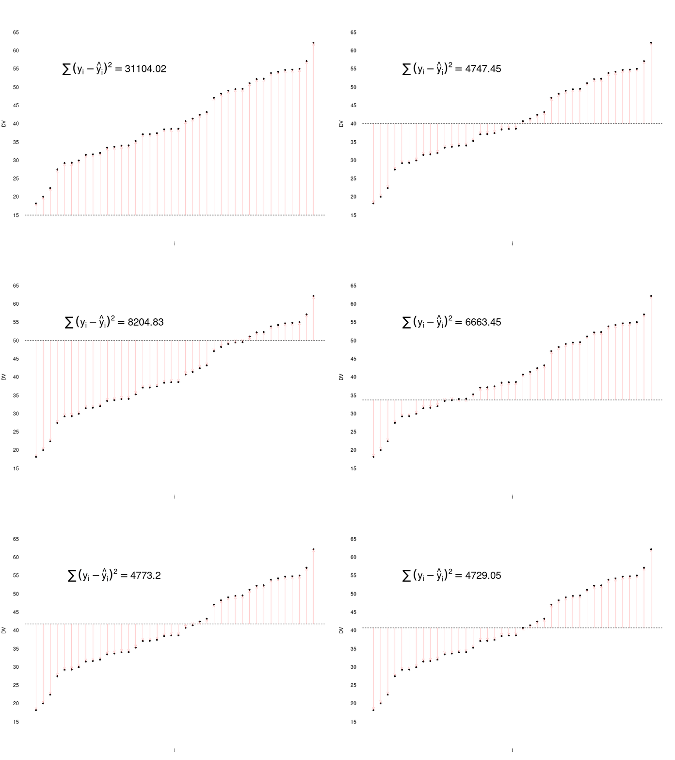
The point that minimizes the squared-deviations is the arithmetic mean!

If we add another variable to the mix we might be able to further minimize the error. For example, if we have a linear predictor/independent variable for that previous dataset, we could try to model the DV as a linear function of the IV, and see if we can find a smaller sum of squares:

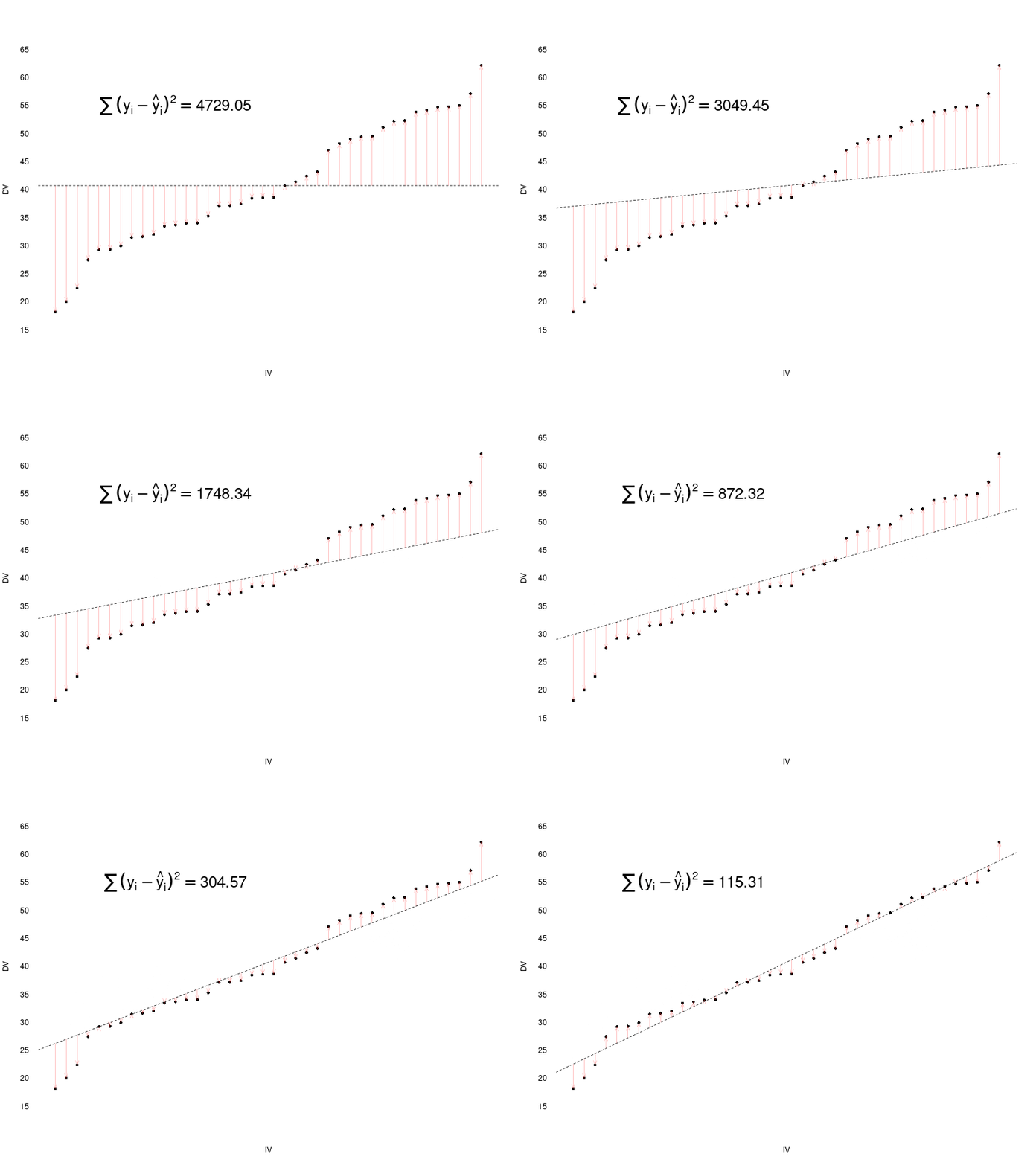
Having the linear predictor variable allows us to reduce the sum of squared residuals a lot.

Variance

The absolute size of the sum of squares depends on the sample size. To get a more general statistic, we can instead calculate the mean squared error (MSE), which is the same thing as variance ($s^2$).

$\frac{\sum_{i=1}^N (y_i - \hat{y})^2}{N} = Var(y) = MSE = s^2$

The square root of the variance is, as we know, called the standard deviation ($s$) or root mean square (RMS). Minimizing the sum of squares is, of course, the same as minimizing the variance/standard deviation. Here we use $s^2$ and $s$ because we are talking about the sample variance and standard deviation.

Why Least Squares?

Least squares has a number of convenient mathematical properties. For one, variance is additive. If you have two independent random variables, $x$ and $y$, then $Var(x) + Var(y) = Var(x + y)$. This property is extremely useful, being the basis, for example, of the ANOVA statistical test.

As we already know, the arithmetic sample mean ($\bar{x}$) is the least squares prediction for a sample and is also a very good (efficient, unbiased, sufficient, etc.) estimate of the population mean ($\mu$). The sample variance ($s^2$) is also a good predictor of the population variance ($\sigma^2$). Unfortunately, unlike the mean, the sample variance is actually a biased predictor—the sample variance will (on average) underestimate the population variance. Fortunately, there is a solution: if we divide the sum-of-squares by $N - 1$ instead of $N$, we get an unbiased estimate of the population variance.

$\frac{\sum_{i=1}^N (y_i - \hat{y})^2}{N - 1} \approx \sigma^2$

In this case, $N - 1$ is the statistical degrees of freedom in our data, which we will learn about more later.

Least squares, like many error/loss functions, is purely a functional heuristic. It is easy to compute and has convenient mathematical properties, but it doesn’t (in itself) mean anything from a theoretical perspective. Conversely, least-squares makes no assumptions about the data. Variance and the mean can be used as inferential “models” of a (normally-distributed) population. However, they are also useful descriptors of the data when there is no model of the population.

Maximum Likelihood

Least squares approaches are useful, but the fundamental core of statistics is another approach to modeling and error functions: maximum likelihood. The idea of maximum likelihood is to find models/parameters that maximize the likelihood of observing our sample data.

Unlike least squares, maximum likelihood requires assumptions about the probability distribution of the data. Typically we assume that:

The population is normally distributed.
The sample data points are independent.
The variance is the same for all data points (even if the mean is different in different groups, for example).

However, maximum likelihood allows us to make other, more sophisticated modeling assumptions, if warranted. For example, other probability distributions (binomial, Poisson, beta, etc.) can be used if they are more appropriate models of our data. There are also ways we can incorporate data dependence or variable variance into the maximum likelihood calculations.

Here’s some data.

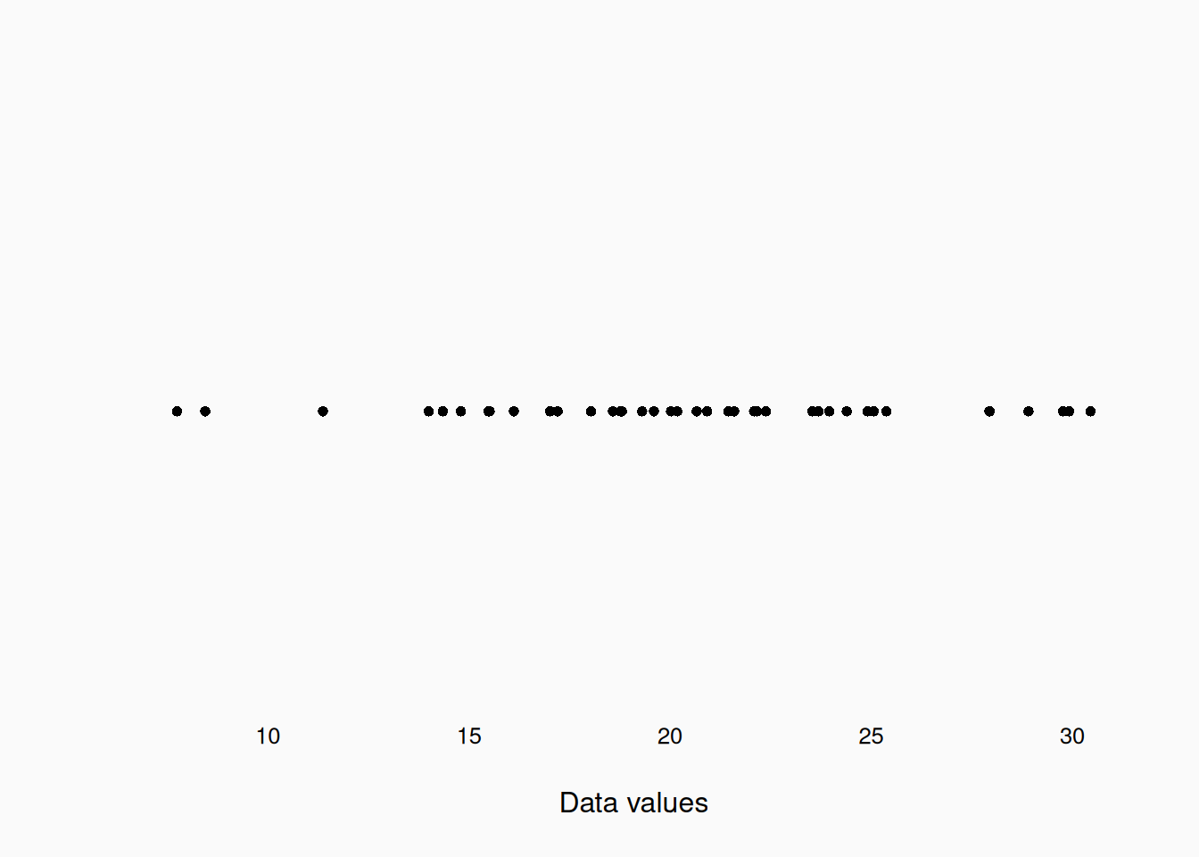
If I assume a particular normal distribution, I can calculate how likely each data point would be, if they were drawn from that distribution.

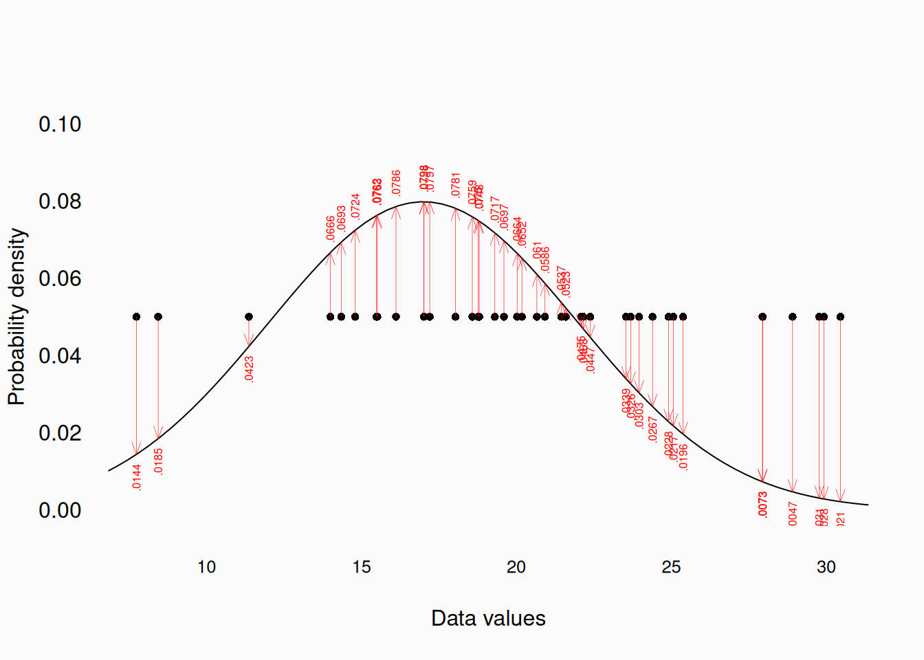
If we assume each observation is independent, the joint likelihood is simply the product of all the individual likelihoods. (See the probability primer appendix.) This is why assuming data independence is so important! If data are dependent, we don’t know what the joint (overall) likelihood is. Unfortunately, the likelihood is usually too small to compute, so we take the log and sum instead. This called the log-likelihood (LL).

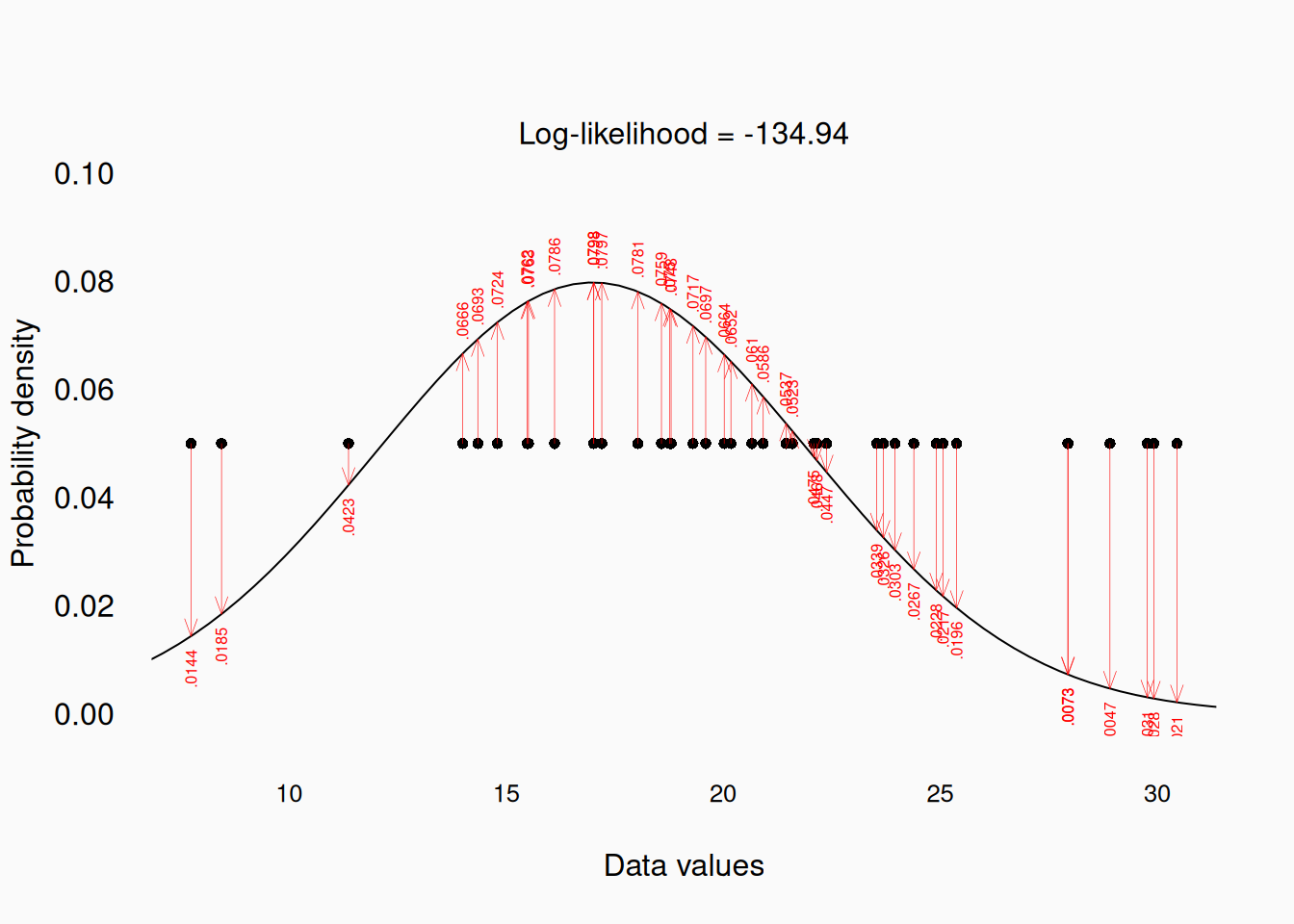
If we maximize the log-likelihood of a normal distribution…

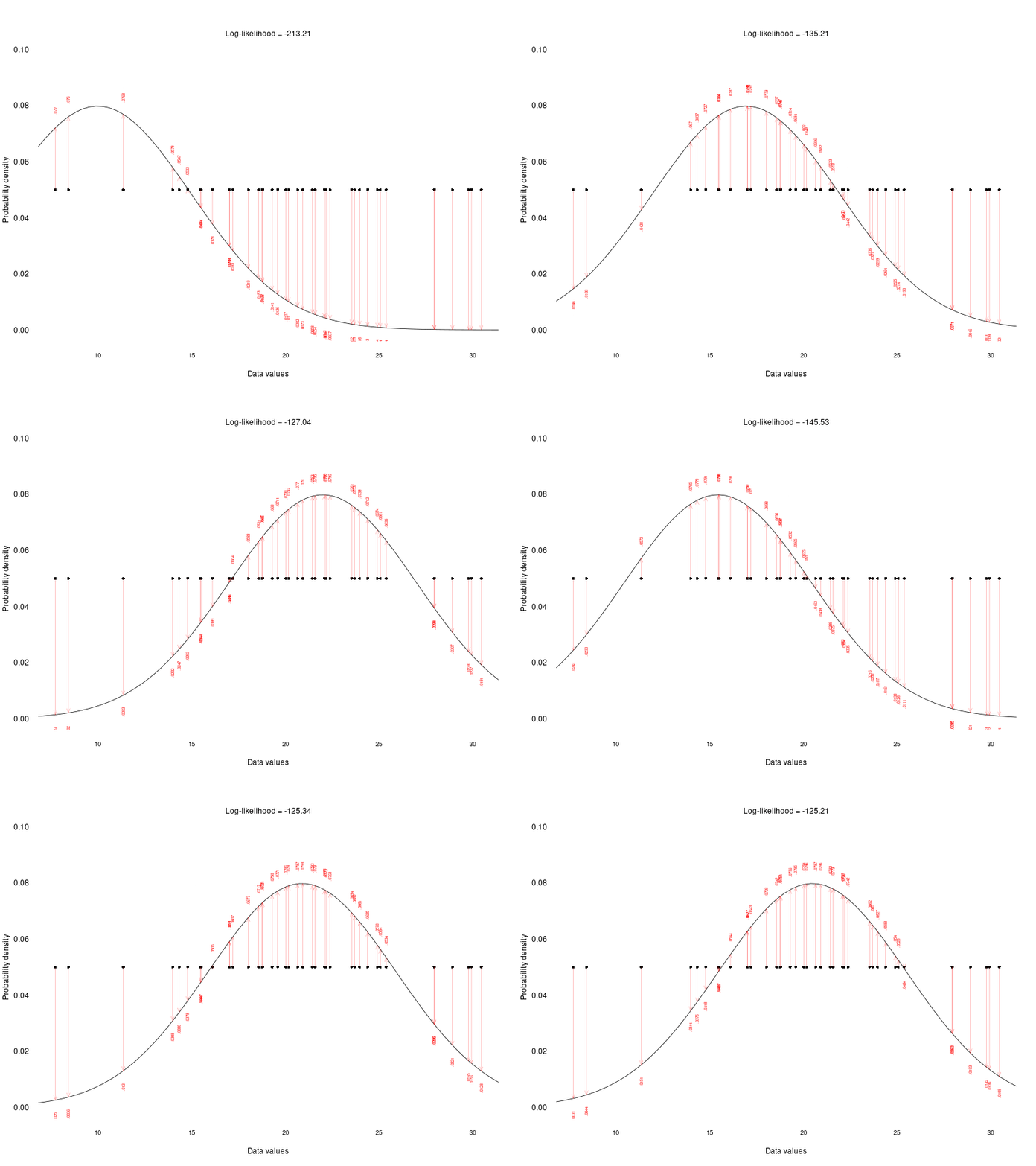
We get the arithmetic mean again! This is only true when we maximize the likelihood of normal-distribution. In general, least-squares estimates are largely valued/used in statistics because they correspond to the maximum-likelihood estimates for independent draws from a normal distribution. This is a big part of why normal distributions are used so much.

Theory

Unlike least squares, maximum likelihood is based on theoretical assumptions about the distribution. If our assumptions are wrong, the maximum likelihood estimates will be wrong. Conversely, accurate maximum likelihood estimates can be more meaningful than least-squares estimates.

For example, for non-symmetrical or bimodal data, the mean and variance can still be computed (least squares) as useful error metrics, but they are a lot less meaningful as models of the data.

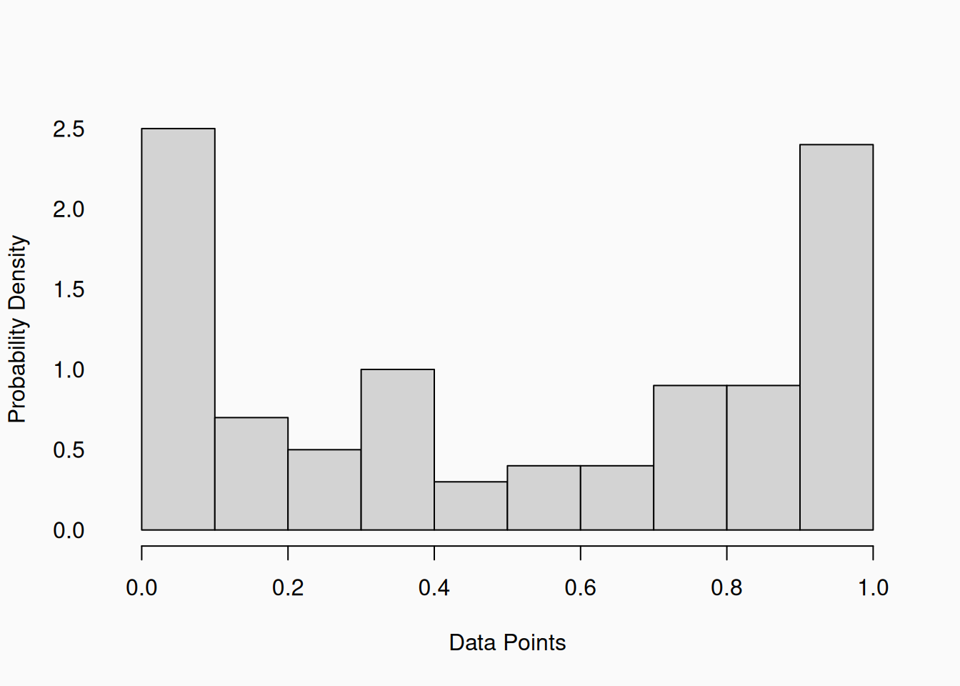
The mean (0.5) of this data is still the point that is “closest” to all the data points—the least squares estimate—, which is useful. However, the data is clearly not normally distributed, and the population probably isn’t either. However, for a maximum likelihood approach, we could model this data using the beta distribution. We could find that the maximum likelihood estimate for this data would follow a beta distribution with parameters $a = .5$ and $b = .5$, which looks like this:

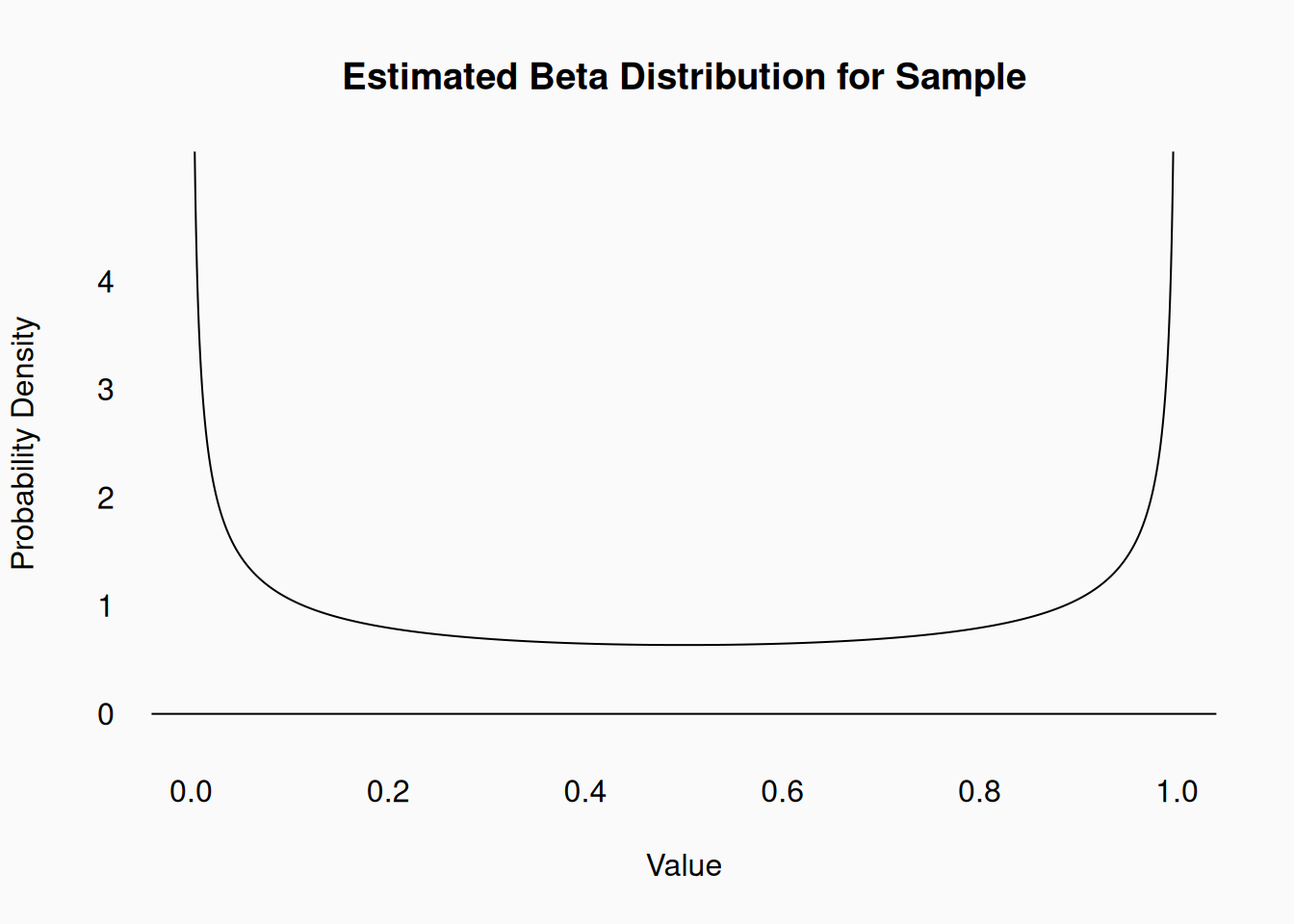
If we use a normal distribution, the maximized likelihood for this data is -41.2. If we use the beta-distribution, the maximized likelihood is 16.15. The beta-based model is a far better fit for this data.

Finding fit

For standard (simple) statistical models, the best fitting statistical estimates are known. That is, we have “analytical solutions” to mathematically derive them. For example, you all know how to compute the arithmetic mean. You now know that the arithmetic mean is the least squares solution, the best estimate of the population mean, and (assuming the data is identically, independently, and normally distributed), also the maximum likelihood solution. Thus, every time you compute the mean of a sample, you can interpret this as “fitting” a (simple, Gaussian) model to the data.

For linear regression equations, the (sample) estimates ($b_k$) for the regression (population) parameters $\beta_k$ can be computed as follows:

$b = \frac{\sum_{i=1}^N (x_{i} - \bar{x})(y_{i} - \bar{y})}{\sum_{i=1}{N} (x_{i} - \bar{x})^2}$

If you use R or Python, for example, to compute a simple linear regression, the software is simply implementing a formula like this. Many other common statistical tests (e.g., ANOVA, $t$-tests) have simple analytical solutions.

When models get more complex, or non-standard, there is no simple solution to calculate the best fitting parameter estimates. This is the case for logistic regression, repeated-measures models, Poisson regression, etc. In these cases, we instead use algorithms to “search” for the best parameter estimates. In machine learning, we call this “training” the model. In statistics, “estimating” or “fitting” the model. Examples of algorithms for model fitting include gradient descent, back-propagation, the expectation maximization (EM) algorithm, and the Metropolis-Hastings algorithm.

Evaluating Fit

How do we judge how “good” a model fits? The most important way is to judge the fit in terms of the constructs and theories being studied. Look at the residual standard deviation ($s = \sqrt{Var(x)}$), which is on the same scale as the data. Imagine that you are researching household income in different communities. You look at the standard deviation in your data and find $s=$$$12_k$. Is that a big range, or a small range? For lower-income people, its a big range. On the other hand if you are trying to use an algorithm to estimate pitch (in semitones) from audio, a standard deviation of $s = 0.1$ will result in music that is noticeably out of tune.

Comparing fit

Of course, there are many more approaches to judging how well a model fits. Generally, this is done by comparing the fit of two (or more) different models.

In least-squares terms, we might ask, “how much does the variance get reduced when we add parameters to the model?” Take the null model ($H_0$) as the baseline, and compute the variance. In practice, this just means, take the mean of the data, with no parameters. We’ll call this $s^2_{null}$. Add your parameters and compute the new variance $s^2_{IV}$. The proportion of the null variance that is “explained” by the model is called the coefficient of determination, or just $R^2$.

Let’s use this example, from above:

When we don’t use the IV, only the sample mean, the residual sum of squares is 4,729. When we incorporate the independent variable (using the linear regression line), the sum of squares is reduced to $115$. In this case, 97.5% of the variance is removed.

$R^2 = 1-(\frac{s^2_{IV}}{s^2_{null}} )$

$1 - (\frac{115.3144}{4729.048}) = .9756$

People will say that the independent variable here “explains 97.5% of the variance in the data.”

In maximum likelihood terms, we can take two models and ask which one has the higher log-likelihood. The difference between the log-likelihoods is the likelihood ratio. The log-likelihoods can only be compared for models with the exact same number of data. (However, if we divide the LL by $N$, to get the cross-entropy, we can compare fits across different data.)

In this case the log-likelihoods are:

$LL_{null} = -139.38$
$LL_{IV} = -91.01$

The difference between these, the (log) likelihood-ratio, is $48.37$. This is a huge ratio, corresponding to a ratio of $e^{48.37} > 10^{21}$—so the linear model is a much better fit.

Over fitting

A fundamental problem is that models with more parameters will always fit better when applied to the same data. Model estimates are, by definition, optimized to fit the data. Sample statistics (e.g., mean) are always closer to the data than the true (population) parameter. This is the problem of over fitting.

Degrees of Freedom

Over fitting is worsened when one parameter estimate depends on another. To illustrate, below I sample 40 data points from a normal distribution with $\mu=10$ and $\sigma^2 = 400$. I can calculate the mean squared-deviation from the sample mean (left panel) and from the true population parameter (right panel):

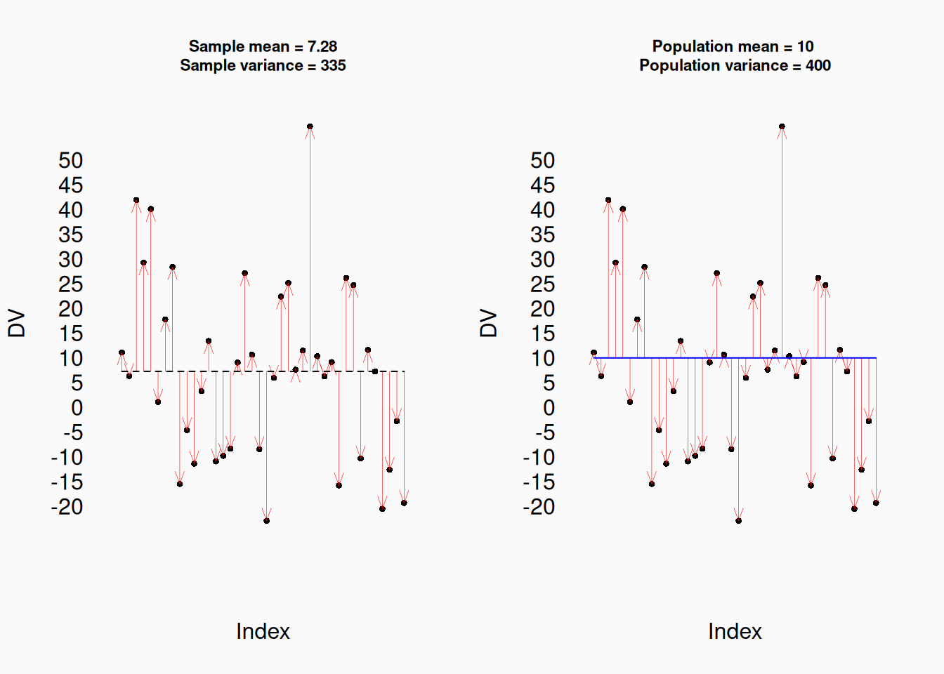
As you can see, the estimate of the variance from the sample is lower (335) than the true variance (400). This will be the case more often than not: the sample variance ($s^2$) is a biased estimate of the population variance $\sigma^2$. Why? Because the estimate of the variance ($s^2$) depends on the estimate of the mean ($\bar{x}$). The sample mean is closer to the sample than it is to the population, so the variance ends up (appearing) smaller.

This will get worse if we add parameters to the model. Maybe half of my data are musicians and half are non-musicians, so I estimate means for each group. This is the same (random) data from above, just randomly divided into groups:

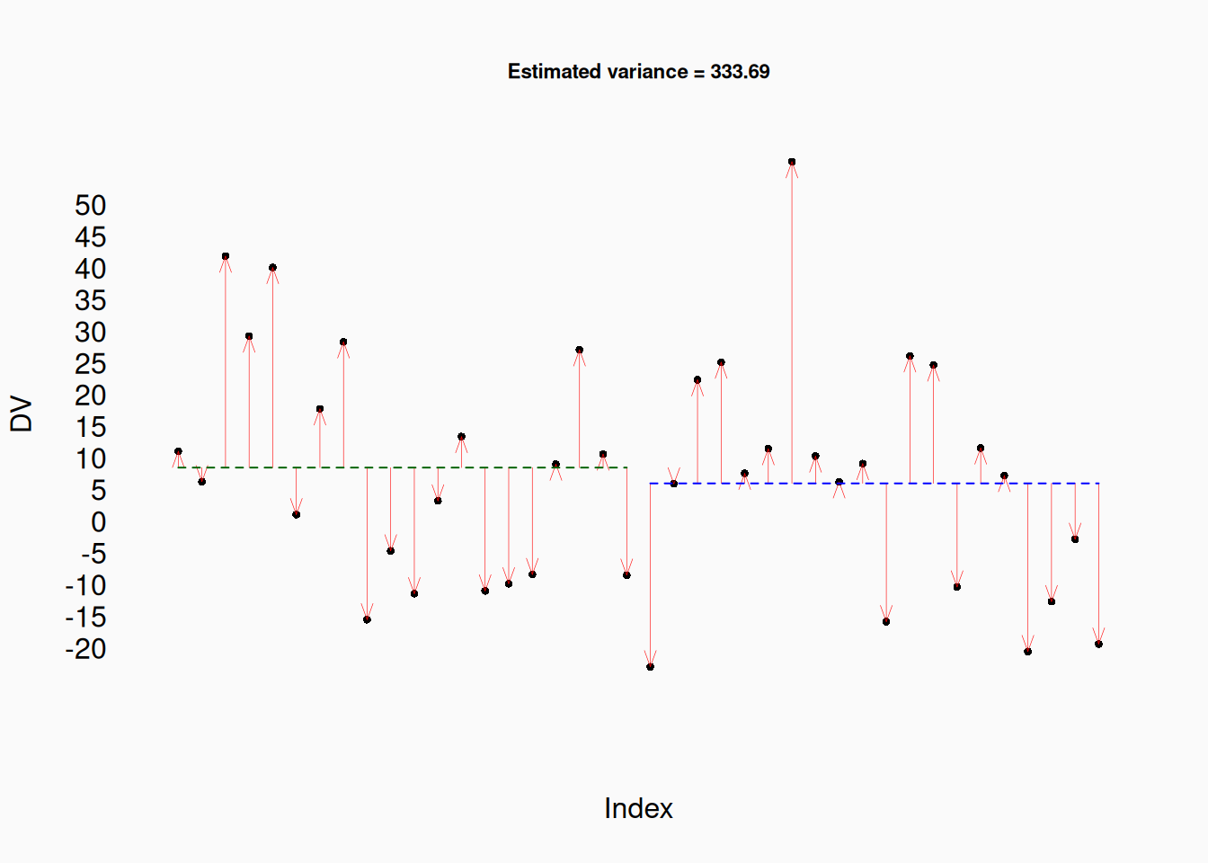
And maybe half of those groups are classical musicians, and half jazz.

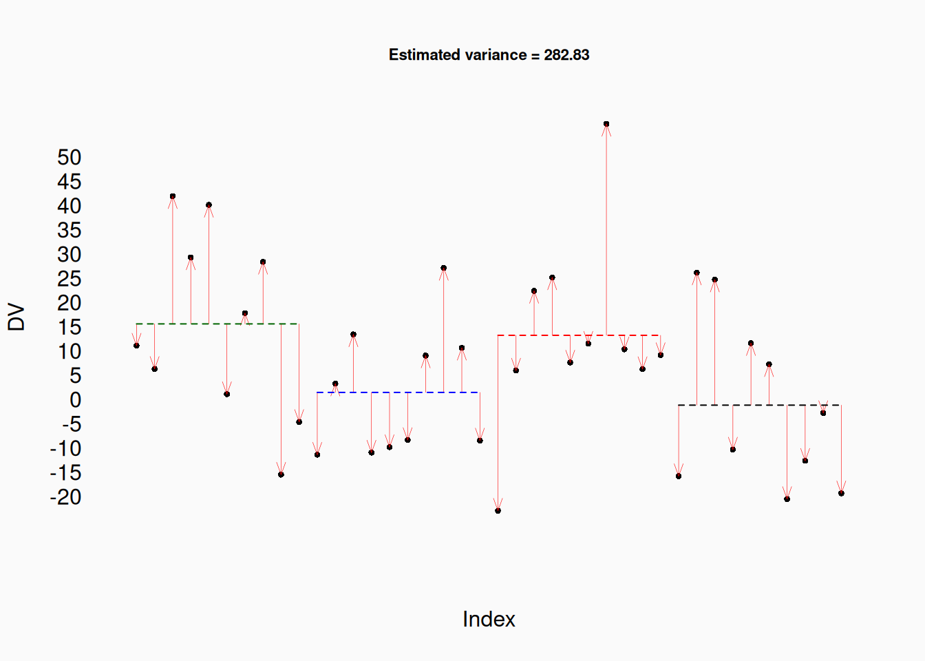
And half are pros, and half amateurs…

Warning in arrows(x0 = 1:40, x1 = 1:40, y0 = mu, y1 = xover, col = "red", :
zero-length arrow is of indeterminate angle and so skipped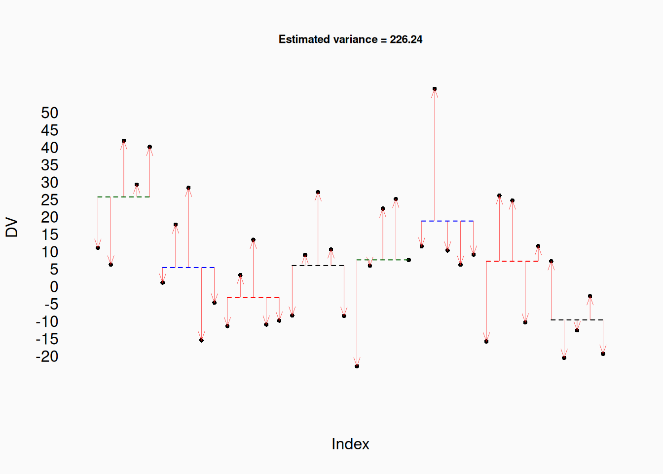

The estimated residual error gets smaller and smaller as we add more means. Again, this is totally random data. None of these groupings are “real” in the population. But if we were working with this sample, we wouldn’t know that. It might appear that the model with more parameters (more groups means, in this case) fits better. But this better fit is guaranteed!

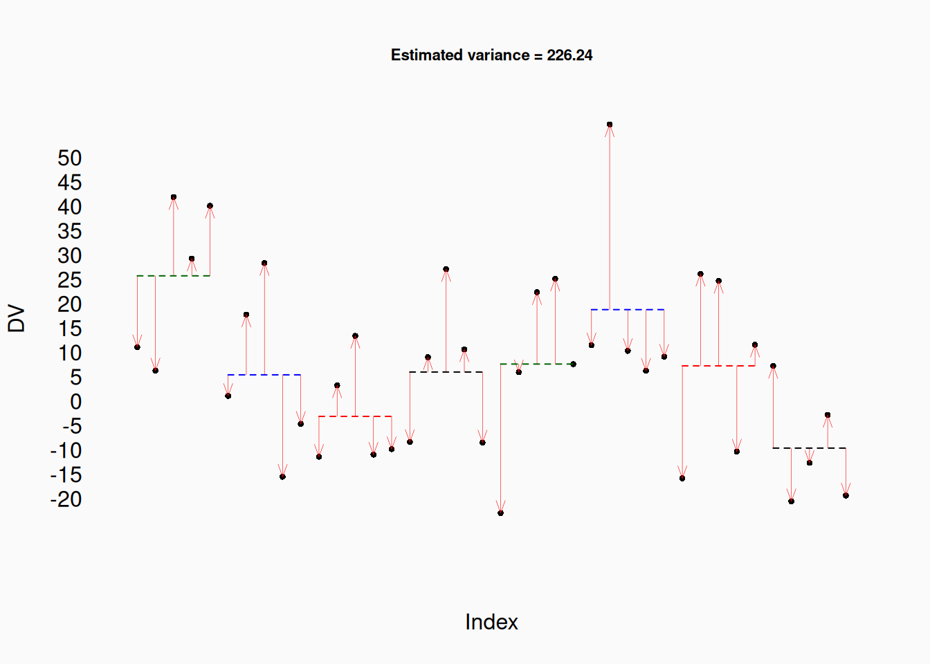
Fortunately, we can account for over fitting (biased) variance. Instead of dividing the sum-of-squared residuals by $N$, we divide by $N-k$, where $k$ is the number of parameters. $N-k$ is called the degrees of freedom.

$\frac{\sum_{i=1}^N (y_i - \hat{y})^2}{N-k} = Var(y) = s^2$

This gives us an unbiased estimate of the true residual variance. Many statistical approaches attempt to correct for over fitting by taking into account degrees of freedom (the amount of data relative to the number of parameters) in some way.

Cross-Validation

The problem of over fitting happens, in part, because we are engaging in double use data—using the same data to fit our models and to test them. This is something I told you not to do! However, it is the standard approach in conventional statistics, and the tests are designed to account for it using things like degrees-of-freedom corrections.

An alternative approach is to explicitly avoid “double dipping” data. Instead fit (or train) the model on one set of data, and test how well it fits on different data. Typically we do this by dividing our sample (randomly) into subsets, and using one subset for training and another for testing. This is called cross validation. We will talk more about this in a future reading.

Note that neither cross validation nor “degree-of-freedom corrections” totally account for over fitting. Over fitting is a pernicious problem in all statistical modeling and machine learning. When models get very complex, they can “learn” to fit the data too well, instead of fitting the population, which is what we want. There is no simple (magic) way to avoid this. The trade-off between model complexity and fit is a difficult balancing act we must always consider.