Appendix B — Statistical Tests
(Modified on 2026-08-12)
743 words
Most statistical tests used in experimental research are based on variations of the general linear model (GLM). The GLM looks something like
\[ Y = link(\beta_0 + \beta_1X_1 + \beta_2X_2 + ... + \beta_nX_n + \epsilon) \]
Where
- \(Y\): Dependent variable(s)
- \(\beta_0\): A “intercept”
- \(X_i\): One or more independent variables
- \(\beta_i\): One coefficient for each independent variable
- \(\epsilon\): An “error distribution”
- \(link(x)\): A “link function” which may (or may not) transform the values to non-linear scale
Such models have, at least, one free parameter \(\beta_0\), one free parameter \(\beta_i\)for each \(X\), and zero or more free parameters for the \(\epsilon\) probability distribution. Here is an example of the GLM which we have already seen,
\[ \text{metal enjoyment} = \beta_0 + gender * \beta + \epsilon \\ \epsilon \sim \mathcal{N}(0,\,\sigma)\\ link(x) = I(x) \]
with one \(\beta_0\), one \(\beta\) and \(\sigma\) used as the standard deviation of the error distribution. (\(I(x)\) is the identity function…i.e., in this case the link function does nothing.)
Variable Types
Most common statistical models are simply linear models with different types of variables.
| Independent variable(s) | Dependent variable | Model |
|---|---|---|
| One binomial | Real \(\sim \mathcal{N}(\mu, \sigma)\) | T-Test |
| One or more categorical | Real \(\sim \mathcal{N}(\mu, \sigma)\) | ANOVA |
| One Real | Real \(\sim \mathcal{N}(\mu, \sigma)\) | Linear regression |
| 2+ Real | Real \(\sim \mathcal{N}(\mu, \sigma)\) | Multiple regression |
| Real and/or categorical | Binomial \(\sim \mathcal{B}(n, p)\) | Logistic regression |
In the GLM, all the variables can be either nominal or numeric (ordinal, interval, or ratio). If the dependent variable is not continuous, or if it is continuous but is “bounded”—e.g, it can only fall in the range [0,1]—we use the link function to map the linear part of the equation onto the nonlinear dependent variable.
Categorical variables are coded as a \(X\) taking on the values 0 or 1. To represent three categorical variables, we need two \(X\), for four categories, we need three \(Xs\), etc. There are actually many ways to code categorical variables: different codings are called “contrasts.” The most common, “treatment” coding scheme, works like this. For the variable fruits with four levels apple, banana, grape, and orange, we’d code them as three \(X\)s, each consisting of zeroes and ones:
| X\(_{banana}\) | X\(_{grape}\) | X\(_{orange}\) | |
|---|---|---|---|
| apple | 0 | 0 | 0 |
| banana | 1 | 0 | 0 |
| grapes | 0 | 1 | 0 |
| orange | 0 | 0 | 1 |
Notice that the apple level doesn’t get its own \(X\) variable: apple becomes associated with the intercept \(\beta_0\) term. (We could choose any of the other levels to be the intercept instead.)
Other approaches to coding
Non-linear effects
Is possible to include curvilinear effects, by raising an independent variable (\(X\)) to a power. For instance, \(X_1^2\). For any of these higher-order terms, it is important to include all lower order terms: i.e., if you include \(X_1^2\), you must also include \(X_1\).
Effect Types
In a GLM, each \(X_i*B_i\) is one main effect. They come directly from your raw data. Another type of effect is an interaction: an interaction is just like any other \(X_i*B_i\) except the \(X_i\) isn’t calculated directly from your data. Rather, the interaction is a new independent variable which is a product of other independent variables: for instance, \(X_i * X_j * \beta_{ij}\). Interactions can be “two-way” (product of two variables), or three- or more-way. An example of a model with an interaction might be:
\[ Y = \beta_0 + X_1\beta_1 + X_2\beta_2 + X_1X_2\beta_3 + \epsilon \\ \epsilon \sim \mathcal{N}(0,\,\sigma)\\ link(x) = I(x) \]
Interactions should never be added to a model unless all their constituent main effects are also included. Interactions between categorical variables end up creating a matrix of all possible combinations of levels. For instance, 2X2 (two variables, each with two categorical levels) GLM looks like this:
| \(X_1 (level 1)\) | \(X_1 (level 2)\) | |
|---|---|---|
| \(X_2 (level 1)\) | \(\beta_0\) | \(\beta_0 + X_1\beta_1\) |
| \(X_2 (level 2)\) | \(\beta_0 + X_2\beta_2\) | \(\beta_0 + X_1\beta_1 + X_2\beta_2 + X_1X_2\beta_3\) |
Common Models (and Tests)
T-test
The Student’s \(t\)-test is based on a GLM with one nominal independent variable with two levels. In other words, there are two groups. The link function is the identity function—i.e., there is no transformation—, so the dependent variable is simply a ratio/interval scale, continuous numeric, value. The error distribution is normal, with only one \(\sigma\) (the standard deviation of the error distribution) used in both groups—i.e., both groups might have different means, but have the same standard deviation. We must also assume that all data point errors are distributed independently (no order effects, no participant effects, etc.)
\(t\)-test is focused on the difference between two group-mean statistics (\(\bar{X}_1 - \bar{X}_2\)) which estimates the difference between the group population parameters (\(\mu_1 - \mu_2\)). The null hypothesis is that \(\mu_1 - \mu_2 = 0\).
Sampling Distribution
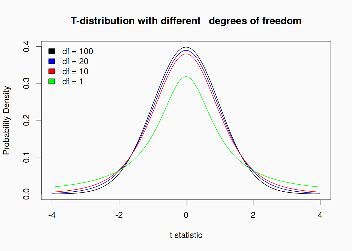
For its statistical test the \(t\)-test makes use of Students \(t\) distribution: As we learned in my Statistical Modeling talk, the sampling distribution for the differences between means (in this case our estimate of \(\mu_1 - \mu_2\)) is a normal distribution with a standard deviation (the standard error) of \(\frac{\sigma}{\sqrt{n}}\). However, in a sample we don’t know what the true population \(\sigma\) is: we can only estimate \(\sigma\) with the sample standard deviation \(s\). This means we can also only estimate the standard error as \(\frac{s}{\sqrt{n}}\). This is where the \(t\)-distribution comes in. The \(t\)-distribution is very similar in shape to the standard normal distribution (\(\mu=0\), \(\sigma=1\)), but has an additional parameter (\(v\)), called the degrees of freedom.
(The larger \(v\) gets, the more like a normal distribution the \(t\)-distribution is.) If we set \(v = n - 1\), then the resulting \(t\)-distribution matches the sampling distribution of sample \(b\)s with $! Thus, we can calculate the \(t\) statistic, as \(t = \frac{\bar{X}_1 - \bar{X}_2}{\frac{s}{\sqrt{n}}}\), where \(t \sim \mathcal{T}({df = n - 1})\). This is exactly what we need to calculate p-values or confidence intervals for \(\bar{X}_1 - \bar{X}_2\).
\(t\)-tests must be one- or two- tailed.
Reporting
To report a \(t\)-test, report the \(\bar{X}_1 - \bar{X}_2\) statistic, the standard error, the \(t\) statistic, and the degrees of freedom.
Simple Regression
The simple linear regression model is based on a GLM with an intercept plus one continuous (interval or ratio) numeric independent variable. The link function is the identity function—i.e., there is no transformation—, so the dependent variable is simply a ratio/interval scale, continuous numeric, value. The simple linear regression thus maps the linear relationship between two numeric variables. The error distribution is normal, with only \(\sigma\) (the standard deviation of the error distribution) used no matter what the independent variable is. We must also assume that all data point errors are distributed independently (no order effects, no participant effects, etc.)
A simple linear regression focuses on a sample statistic \(b\), which is an estimate of the population statistic \(\beta\), which represents the “slope” of the line which maps between the two variables. The null hypothesis is \(\beta = 0\).
In a simple linear regression, \(b\) is closely related to Pearson’s \(r\): \(r = \frac{bs_Xs_Y}{s_X^2}\). Pearson’s \(r\) is the “standardized” version of \(b\).
Sampling Distribution
Like the difference between sample means in a \(t\)-test, an estimate for the standard error of \(b\) can be calculated, with \(\frac{b}{SE} \sim \mathcal{T}(df = n - 2)\). We can thus calculate confidence limits and p-values for \(b\).
Reporting
To report a simple linear regression, report the \(b\) statistic, the standard error, the \(t\) statistic, and the degrees of freedom.
One-way ANOVA
A one-way Analysis of Variance (ANOVA) is based on the GLM with one nominal independent variable with more than two levels (call the number of levels \(k\)). The link function is the identity function—i.e., there is no transformation—, so the dependent variable is simply a ratio/interval scale, continuous numeric, value. The error distribution is normal, with only one \(\sigma\) (the standard deviation of the error distribution) used in both groups—i.e., both groups might have different means, but have the same standard deviation. We must also assume that all data point errors are distributed independently (no order effects, no participant effects, etc.)
ANOVAs are focused on the differences between more than two group-mean statistics (\(\bar{X}_1, \bar{X}_2, ...,\bar{X}_k\)), which estimate the differences between the group population parameters (\(\mu, \mu_2, ...,\mu_k\)). The null hypothesis is that \(\mu_1 = \mu_2 = ... = \mu_k\). Since the null hypothesis is that all means are equal, even one different mean is enough to reject the null hypothesis. This means that in an ANOVA with eight levels, seven means could be equal while one is different, and this would mean we’d reject the null hypothesis. The ANOVA is thus an “omnibus” test. It is very common to follow up an ANOVA with “multiple comparisons” between the various groups using \(t\)-tests. When we do this, the Tukey multiple comparisons procedure should be used to correct for multiple NHSTs.
Sampling Distribution
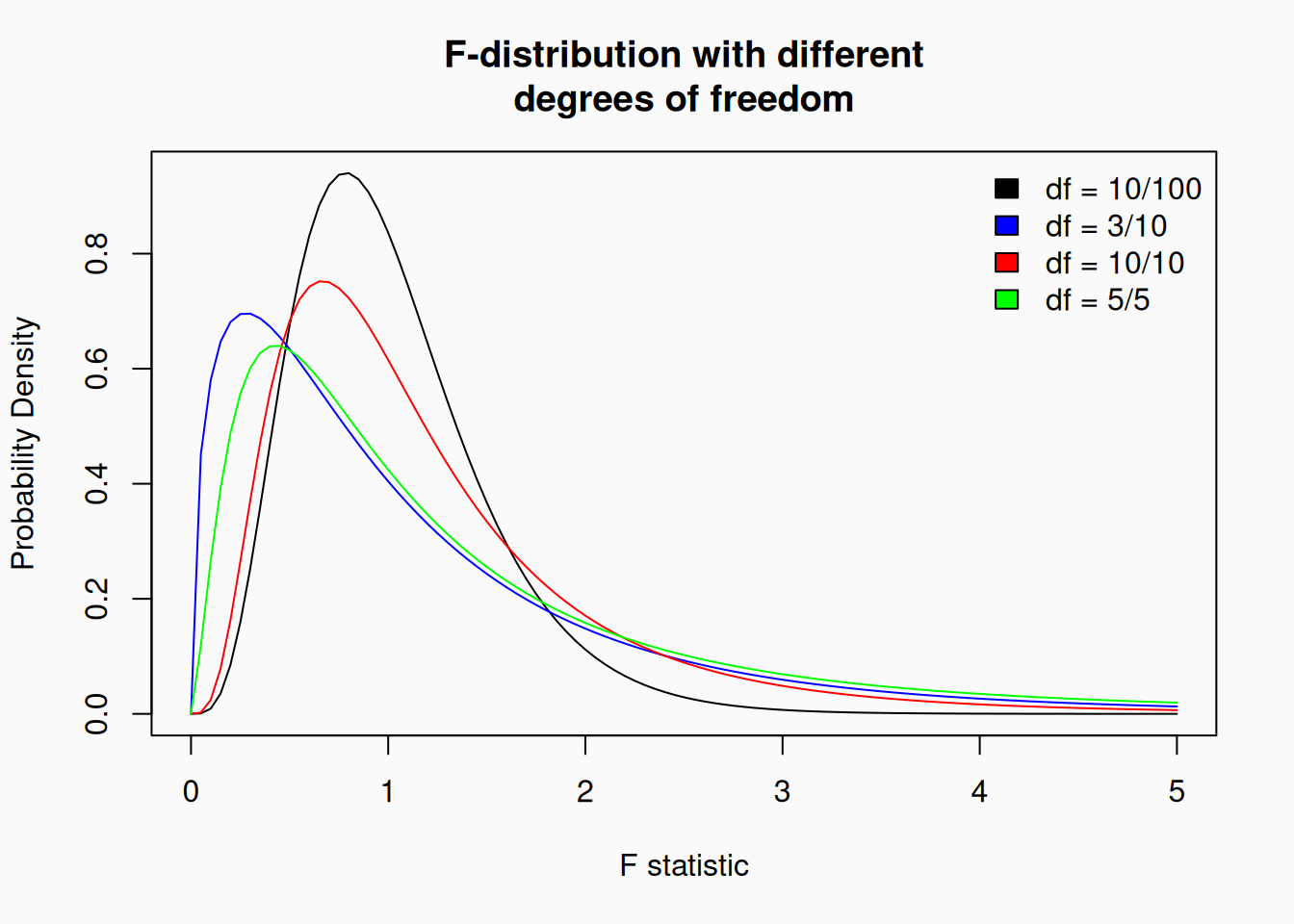
The ANOVA test is not based on any parameter estimate in the model, but instead on a statistic (\(F\)) calculated based on the variance in the model—hence, the “analysis of variance.” The \(F\) statistic is the ratio between two different estimates of the residual error \(\sigma\) from the data. One estimate, the within-group variance is estimated from the distribution of data points within the groups (\(df = n - 1\)). The other estimate, the \(between-group variance\) is estimated from the variance of the group means (\(df = k - 1\)). The statistic we use is \(F = \frac{\text{variance between groups}}{\text{variance within groups}}\). The logic is, that if the null hypothesis is true, these two estimates of the variance should be about the same, so \(F \approx 1\). In fact, if the null hypothesis is true, \(F\) follows the \(F\)-distribution, a probability distribution with two free parameters: \(df_1\) and \(df_2\). As you might have guessed, we use \(df_1 = k - 1\) and \(df_2 = n - k\) to parameterize the correct \(F\)-distribution.
Reporting
To report a one-way anova report group means (\(\bar{X}_1...\bar{X}_k\), the \(F\) statistic, and both the degrees of freedom (for the numerator and denominator of \(F\)).
Simple Models Summary
\(t\)-tests, simple regressions, and one-way ANOVAs are closely related versions of the GLM. The \(t\)-test and simple regression both estimate \(t\)-statistics, which follow a \(t\)-distribution, while ANOVA uses a \(F\)-statistic and \(F\) distribution. In these simple cases, \(F = t^2\)! (It is indeed possible, to test either \(t\)-tests or simple linear regression using and \(F\) test instead of a \(t\)-test, though this is not commonly done!.)
As another parallel, the \(\bar{X}_1 - \bar{X}_2\) statistic in a \(t\)-test can be normalized, like the \(b\) statistic in a simple regression, resulting in a \(r\), correlation coefficient! What’s more, we can then calculate \(r^2\) for either model. \(r^2\) represents the “proportion of variance explained by the model”—you might guess that we can also calculate \(r^2\) for an ANOVA model (but not \(r\))! \(r^2\) thus gives us a standardized way to compare the effect size of these three simple models.