55 Effect Size

(Modified on 2026-08-11)
1,650 words

When analyzing data, we spend a lot of time estimating the “true” relationships between variables, characterizing and visualizing them, and especially testing whether they are or aren’t “null” (NHST). Doing all this work, it can be easy to lose track of the big picture. The real question we want to answer is: do the relationships we observe matter? Do they matter to our theories? Do they matter in practice? To put it another way, we want to know how strong the relationships we observe are, and whether they are strong enough that we—or our readers—should really care about them.

The strength of a causal effect is called the effect size, and we will use this same term to describe correlational relationships as well. Like everything in good research, interpreting effect size requires careful thought. There is not one correct way to describe the size of an effect; It depends on the nature of our research variables and the amount of error we observe.

Don’t forget to also consider the direction of effects: i.e., is the correlation positive (vary together), or negative (vary in opposition)?

But wait… Aren’t statistical tests supposed to determine whether an effect matters? Isn’t that why we do null hypothesis significance testing (NHST)? Not exactly. Significance tests are a crucial first step in data analysis, because they are the main point where our hypotheses can be falsified—creating a bottle-neck on type-1 errors. If a test is not significant, we are forced to acknowledge that our data could be potentially explained by random chance. If a test is significant, we are cleared to make the claim that the null hypothesis is false. However, this alone doesn’t mean we can make a strong claim about our findings.

A significance test is the first step in data analysis, not the final word. The final word should be about the effect size.

Recall that the null hypothesis is (typically) that the effect parameter we are testing is exactly zero. If a parameter is not zero, the null hypothesis is false, even if the effect is really, really tiny. Even if the effect is tiny, you can still (potentially) see a significant NHST. It’s thus very important to distinguish “statistical significance” from real-world “significance.” A significance test is the first step in data analysis, not the final word. The final word should be about the effect size.

In practice, the most useful pieces of information we report to our readers are estimates, and especially visualizations, of the magnitude and direction of the relationships we observe between our research variables. Each of these reports should be accompanied by a null hypothesis significance test; For any non-significant effect, we must accept that the true effect could be zero, and there is no point in interpreting the observed effect size—our conclusions should be (generally) that we can’t claim there is any effect. On the other hand, if a test is significant, we should then spend some time interpreting the effect size, and use this to make more specific conclusions. If a statistically-significant effect size is very small, we should point this out. If the effect is much smaller than what we predicted, a priori, we should point this out. We might even reject our research hypothesis, even if the statistical test was significant.

Remember, the effect sizes we observe in a sample of data are just estimates. Also, correlational or causal relationships between multiple variables can often obscure true relationships. This means that, for example, an effect size might appear weak simply because there are some confounding elements that haven’t been properly controlled. It is possible that, with the right controls, an apparently small effect will turn out to be a big effect that was diluted. This is why it is important to visualize different combinations of variables in different plots, and to build statistical models which control for correlations between different independent variables.

Reporting Effect Size

There are a number of ways to report the effect size, and plenty of disagreement between scholars on which is best. The simplest, and probably best, way to communicate effect sizes is with plots. A plot (with appropriate x-axis and y-axis scaling) will give your readers an immediate sense of how large the effect is. Of course, we generally also want to report effect-size statistics as well—below I discuss a number of standard statistics. However, there is no reason to limit yourself to one “correct” report: Report the effect size in as many ways as you can. Your goal is to transparently convey an intuitive sense of how strong the effect is, and this can often be done best by comparing multiple viewpoints.

It’s all relative

How do we know if an effect is big, or important? Well, it’s all relative.

Relative to the scale of variables.
- A change of +2 is big on the scale of GPA (grade point average), small on the scale of beats-per-minute, and tiny on the scale of yearly income.
Relative to your theoretical expectations.
- What kind of effect size did you expect?
Relative to practical applications.
- How many lives will your new medication save? One in a million? One in a thousand?
- How many more users will download your new software? 10 per month? 1,000 per month?
- How different is the average tempo of Thrash metal and Gloom metal? $2_{bpm}$ or $50_{bpm}$?

These considerations are paramount. Usually, this means reporting, graphing, and interpreting effect sizes on their original scale, which is the most ecologically valid and intuitive in practical/theoretical terms.

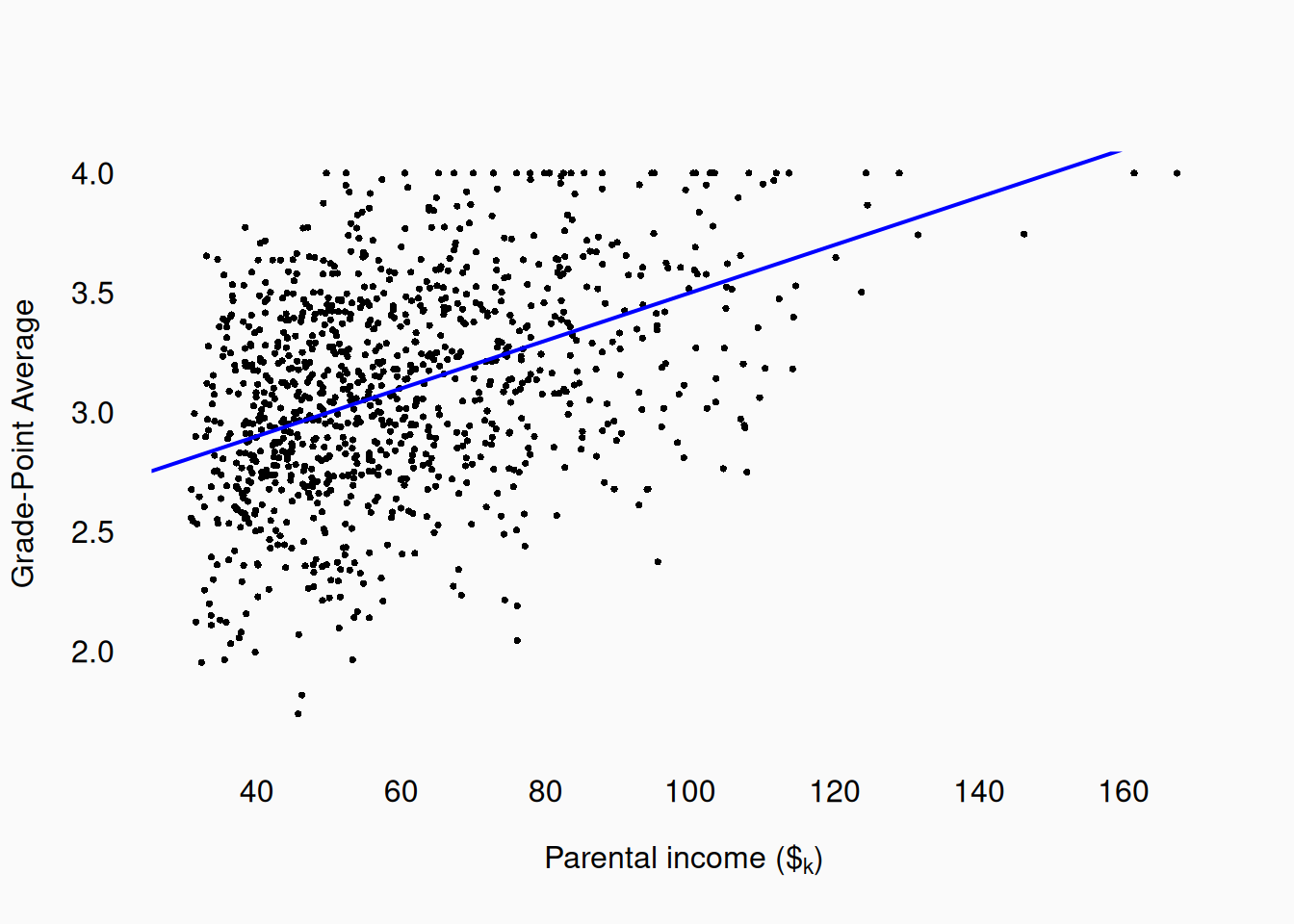
Let’s consider a hypothetical example, predicting university-student grade point average (GPA) using parental income. Imagine that we gather data and find that every $$1_k$ increase in parental income predicts a $+0.01$ increase in students’ GPA. If you know what GPA is, and you know what $$1_k$ income feels like in the real-world, you can pretty quickly get a sense of what the relationship is—you can intuit for yourself whether this is a strong or weak effect. To increase GPA by $0.5$ you’ll on average need a $$50_k$ boost in income. This would mean that students from even upper-middle class families (perhaps make $$150_k$ per year) would (on average) have a pretty significant GPA advantage over students from lower-middle class families (perhaps making $$50_k$ per year).

Error

From a methodological perspective, there is one other overarching concern to consider: How big is an effect relative to the variability in the data? For example, imagine that we measure the preferred practice tempos of male and female musicians. Here are two hypothetical samples, measuring practice tempos across male and females:

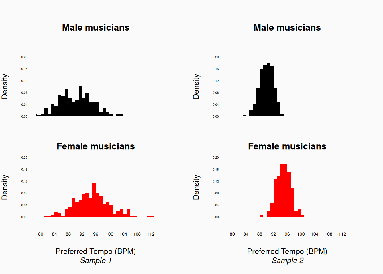
Here, the left two plots show one sample, and the right two plots another sample. Both samples show the same difference between male and female musicians: an average difference of about five beats-per-minute (bpm). Is a difference of five a big, or important difference, in meaningful terms? That is up to us (and our readers) to decide or argue. However, we can also compare this difference to the variation we observe: our left sample shows a lot of variance, with a considerable overlap between the male and female samples. In contrast, in the right sample, the male and female musicians overlap much less. This means that, compared to the error, the right sample has a bigger effect size.

Generally, you should always report effect size in the context of error, so that your readers can better judge the effect size for themselves. For example, for the samples of data above, it would be bad to just show this:

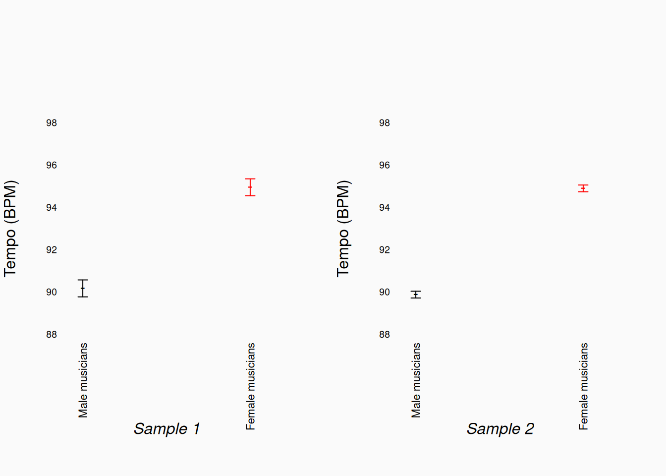
This plot shows the means, and confidence intervals for the means, of the same male/female preferred tempo data above. However, these plots don’t actually show the full distribution of data points, and the difference in relative effect size is not nearly as apparent here! The full histograms (above) give us a much better picture of the effect size.

Now, there is no one “correct” way of thinking about effect size in the context of error. For one thing, it depends on the nature of the error. Look at the left-side tempo histograms above (Sample 1), and consider this: do the values here really represent variation between musicians? For example, are there really some male musicians who prefer $84_{bpm}$ and others that prefer $112_{bpm}$? If so, that variance may be relevant to our hypothesis/theories, and the conclusions we want to make. In this case, it would make sense to consider the effect size only relative to the error.

In contrast, maybe the variance we see here is really just measurement error: maybe for Sample 1 we measured tempo preferences by estimating the tempo from accelerometer data from musicians’ smart watches and the measurements are really just inaccurate. Maybe all musicians really prefer tempos in the range $92$–$96_{bpm}$, and the higher/lower values we are seeing in the first Sample 1 are just random noise. In this case, considering the effect size relative to the error is misleading: the “raw” effect size of $\approx$ five bpm difference is more meaningful, even though there is a lot of error.

Standardized metrics

In the previous section, we talked about considering effect size “relative” to error. This is something we can and should, do intuitively, as we interpret graphs (as above). However, it is also common to do this quantitatively, by scaling our effect size statistics relative to their variance. The basic approach is to divide effect statistics by the estimated residual standard deviation. This creates a standardized statistic. Standardized statistics exist on an abstract scale, in “units” of standard deviations; One advantage of using standardized statistics, is that they are easier to compare with other analyses, even involving variables measured on radically different scales. Disadvantages of standardizing statistics include that we lose the connection to the “real-world” measurement scale, and that different sources/types of error are conflated.

A common standardized metric is Cohen’s $d$. Cohen’s $d$ is simply the difference between two sample means, divided by the residual standard error.

\[ d = \frac{\bar{x} - \bar{y}}{s} \]

In the case of our two preferred-tempo samples above, the Cohen’s $d$ estimates are 0.95 (Sample 1) and 2.38 (Sample 2).

We already saw some examples of standardized statistics in the linear models chapter. The most significant of these is Pearson’s correlation coefficient ($r$), which is the covariance standardized by the standard deviations of both variables. $r$ ranges between $-1$ and $1$, with $0$ being no correlation. Don’t ignore the sign!: $r = .5$ and $r = -.5$ are two different correlations, with the same absolute strength but opposite directions.

Consider again our income-GPA data mentioned above, where we said that a $$50_k$ increase in income predicted a $+.5$ increase in GPA. If we measure income on scales of $$1_k$ dollars, the relationship between income and GPA we have observed has a regression slope of $b = .01$. To standardize this, we need to know the standard deviations of each variable. The standard deviation of parental incomes is $20_k$; The standard deviation of GPA is $0.4$. The fully standardized effect of income on GPA is then

\[ b * \frac{s_{income}}{s_{GPA}} = .01 * \frac{20}{.4} = 0.5 = r \]

Interpretation

Standardized statistics are useful because they allow us to compare statistics across studies, including past studies. After seeing these same metrics in use in many studies, we can start to form some intuitions about how “big” they are. In fact, you’ll often see ordinal heuristics for interpreting standardized statistics, like:

Pearson’s $r$
- $.1 < |r| < .3 \implies$ small
- $.3 < |r| < .5 \implies$ medium
- $.5 < |r| \implies$ large
Cohen’s $d$
- $.01 < d <= .2 \implies$ very small
- $.2 < d < .5 \implies$ small
- $.5 < d < .8 \implies$ medium
- $.8 < d < 1.2 \implies$ large
- $1.2 < d \implies$ huge

These sorts of standardized interpretations should be taken with a grain of salt! Many researchers are way over confident in their “feel” for values like $r = .32$. Remember Anscombe’s quartet (1973)?:

Each of these datasets has the same $mean(x)$, $Var(x)$, $mean(y)$, $Var(y)$, $r$/$r^2$, and $b$! Just because standardized metrics are familiar doesn’t mean that they are automatically interpretable. Using standardized statistics can give us a false sense of familiarity and security. Always plot your data!

Coefficient of Determination

Another common effect size is the coefficient of determination: $r^2$ (or sometimes $R^2$), pronounced “R squared.” In simple regressions (between two variables) the coefficient of determination is indeed Pearson’s $r$ squared. $r^2$ ranges from 0 to 1, and indicates the proportion of variance “explained” by the linear model.

\[ r^2 = 1 - \frac{Var_{residual}}{Var_{total}} \]

This means that it is literally a representation of effect size purely in terms of error.

In our parental income-GPA example, $r^2 = 0.5^2 = .25$. Only about 25% of the variance in GPA is “explained” by parental income.¹

Sample Size

Effect size is important because, really, it’s the thing we want to know. However, effect size is also an important methodological consideration, as it strongly influences the sample size we need. If the effect size is large relative to the error, you can make valid claims with surprisingly little data.

In fact, it is a common mistake to knee-jerk criticize research for having too little data. Strong—important—effects can be detected reliably using little data. If you find a statistically significant effect using a small sample, the effect must be large; this means that conclusions made with (relatively) small sample sizes are, in some respects, more compelling. Conversely, if you have a very large sample, you might end up finding statistically significant effects that are actually very small and uninteresting.

This doesn’t mean small samples are good! We want larger samples to improve the reliability, accuracy, and generalizability of our research. The main lesson here is that very large samples—with hundreds of human participants, or millions of pieces of music—are not all they are cracked up to be. As we’ve discussed elsewhere, increasing the sample size beyond a point has little advantage. The new lesson is that using very large samples can lead us to making claims about effects that are actually very weak. In some ways, a moderately-sized sample can be a “sweet spot”: large enough to be reliable, but small enough that only meaningful effects are likely to shine through.

Of course, the flip side of this is that small samples won’t allow you to make claims about subtle effects and relationships. The sample size needed to make a research claim, given a relative effect size, can be determined by calculating the statistical power.

Not P values!

Calculating $p$-values is an essential part of the null hypothesis significance test (NHST) procedure. However, $p$-values themselves are not good measures of effect size. They are not statistical estimates of anything; Rather, they are highly variable descriptions of the sample based on the null-hypothesis assumption. If the null hypothesis is false, $p$-values are meaningless. Small changes in the data can cause large changes in a computed $p$-value.

If the null-hypothesis is true, $p$-values are uniformly distributed between 0 and 1. However, if the null-hypothesis is false, $p$-values are affected by two things:

The effect size.
The sample size.

This means that a small $p$-value may mean you have a strong effect or that your sample size is large relative to the effect. With a very large sample size, it is quite likely that you’ll encounter some very small $p$-values. However, this doesn’t mean that your effect size is large, or that your finding is important. Statistical significance does not imply research significance.

Unfortunately, it is very common to report $p$-values in a way which is interpreted as an effect size. You’ll see papers report things like..

$p < .01$
$p < .001$
$p < .00000001$

This is a bad practice, because those cut-offs were not chosen a priori. Using (implicitly) a lower $\alpha$ when the $p$-values happens to be small actually undermines the whole NHST procedure. In all these tests, the a priori was $\alpha = .05$; if the $p$-value was $p = .04$, the researchers would have reported a significant result. The NHST is sensitive to what we would do in every scenario. If $\alpha = .05$ is the cut off we would use, not $.01$ or $.0001$.

If we report things like:

$p < .01$
$p < .001$
$p < .0001$
$p < .00001$
$p < .000001$

All we are really doing is reporting the $p$ value rounded to the nearest power of 10. But $p$-values are bad metrics of effect size, and reporting $p$-values rounded to the nearest power of 10 doesn’t change that fact.

This is assuming a linear relationship of course. A non-linear relationship might account for more variance.↩︎