| Population parameter | Sample Stastic | |||
|---|---|---|---|---|
| Mean | \(\mu\) | “myew” | \(\bar{x}\) | (“x bar”) |
| Variance | \(\sigma^2\) | “sigma squared” | \(s^2\) | |
| Standard deviation | \(\sigma\) | “sigma” | \(s\) | |
| Linear coefficient | \(\beta\) | “beta” | \(b\) | |
| Correlation | \(\rho\) | “row” | \(r\) |
46 Statistics
(Modified on 2026-08-11)
1,770 words
If we take a sample of data and compute any numeric value from it, this is called a statistic. There are three main ways statistics are used: description, inference, and evaluation (testing). We will talk about the last case, test statistics, in a later reading.
We can use statistics to describe our sample. Descriptive statistics cannot be right or wrong; They don’t make any assumptions or make claims. They simply communicate useful information about your sample to your audience. If you have a sample of human participants, you can tell your readers that their average age was 22.4 and the range of their ages was 19 to 28. Descriptive statistics serve the same uses as data visualization, and we often use descriptive statistics in data visualizations.
The central concern of the field of statistics is how sample statistics relate to population parameters.
The main goal of statistical analysis is not just description but inference. Specifically, we want to use our (sample) statistics to make inferences about the population we sampled from. We consider an inferential statistic to be an estimate of the true value of a parameter in the population (i.e., the data-generating process). The central concern of the field of statistics is how sample statistics relate to population parameters.
Many common statistics are used in both descriptive and inferential ways, often simultaneously. The best example is the expected value, a.k.a. the (arithmetic) mean: The mean is a very useful descriptor of the central tendency of any numeric sample on an interval or ratio scale.1 The mean of a sample (\(\bar{x}\)) is also a very good estimate of the mean of the population (\(\mu\)) that the sample was drawn from.
Notation
Conscientious researchers and instructors will use consistent mathematical notation to differentiate sample statistics from population parameters. Usually we use Greek letters for population parameters and Roman letters for sample estimates. The main examples used in this book are:
Unfortunately, these distinctions aren’t made consistently among scholars, so watch out for various notations!
Estimation
Generally, we want statistics which are good estimates of corresponding population parameters. What makes a statistic a “good” estimator? There are a number of common criteria:
Unbiased: Unbiased statistics will be centered around the true population parameter. In other words, an unbiased estimator will come out above or below the true value equally often, not biased one way or the other. If a statistic is unbiased, then the expected value (mean) of the statistic will be the population parameter.
Consistent: A consistent estimator will converge toward the true population parameter as the sample size is increased. More data, more accuracy.
Efficient: This is an obvious one—an efficient statistic tends to be close to the true population parameter.
Sufficient: A sufficient statistic gives us all possible information about the parameter from the sample. Once you’ve calculated a sufficient statistic, no other statistic or calculation from the same sample can improve the estimate.
Robust: A robust statistic works well for a wide range of probability distributions, under a wide range of assumptions. This means that it will still be a good estimate even if the data violates some of the assumptions we are making.
Insensitive: The value of a sensitive statistic can change a lot given small changes to the sample. For example, the median is a measure of central tendency that is insensitive to small changes in a sample.
For example, if you have ten people with a mean salary of $\(65_k\) per year and you add one person with a salary of $\(400_k\) per year, the mean is “pulled up” to $\(95_k\). In contrast, the median is much less sensitive to such changes: the median value would remain close to $\(65_k\).
We can now start to fully understand the value of the sample mean (\(\bar{x}\)): The sample mean ({x}) an unbiased, consistent, and sufficient estimator of the population mean (\(\mu\)). This is true for all probability distributions, so it is also quite robust. For data sampled from normal distributions, \(\bar{x}\) is also the most efficient estimator of \(\mu\). The only weakness of the sample mean is that it is highly sensitive to extreme values.
Sampling Distribution
In the Random Variables chapter, I introduced the idea that we can model measurement error as “draws” from probability distributions. We extend this model to larger samples of data—simply imagine that we are drawing multiple independent values from the same probability distribution. We can then calculate statistics from this random sample of numbers.
Every time we sample a random variable, we’ll get different numbers and our sample statistics will be different. However, if we know—or assume that we know—the (population) probability distribution that generated the sample, we can use that knowledge to calculate how likely observing each data point, or statistic, would be. Thus, the (hypothetical) probability distribution becomes our model of the real-world data-generating process.
For example, consider the distribution of adult American men by height. We can model the “true” population of adult heights by assuming it follows a normal distribution—this is definitely not a perfect model of this population, but it may be close enough to be useful (All models are wrong, but some are less wrong). Let’s imagine that this population has a mean \(\mu = 175.3_{cm}\) and a standard deviation of \(\sigma = 7_{cm}\). If we randomly sample ten American men, and measure the mean height of the sample we might see something like \(\bar{x} = 174.2_{cm}\). If we sampled a different ten men, we might see \(\bar{x} = 176.57_{cm}\). Each sample will have a different sample mean, and never be quite the same as the population parameter.
So we took two different samples and got two different sample means. What would happen if we kept taking more random samples of ten men, and calculating their average height over and over again? Say, one thousand times? This is what it would look like:
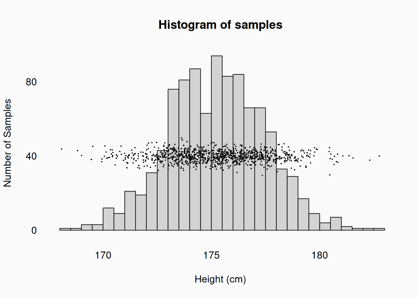
This is called a sampling distribution: in this case, the sampling distribution of the \(\bar{x}\) (sample means). A sampling distribution is not the distribution of the raw (individual) data points: its the distribution of the statistics calculated from the raw data. In this hypothetical scenario, we have measured the height of \(10 * 1,000\) men, but we aren’t looking at the distribution of all 10,000 numbers, we are looking at the distribution of the 1,000 statistics (one mean per sample).
By looking at the sampling distribution, we can confirm a few properties of the sample mean we mentioned above:
The distribution is centered around the true population mean (\(175.3_{cm}\)), which means the statistic is unbiased;
Of course, with these one thousand samples of 10 men, there are some pretty extreme groups that arose entirely due to random sampling error: one sampled group had a mean of 182.75\(_{cm}\)!
The distribution, even though the sample size each time is only 10, is fairly tightly packed around the population mean, so the statistic is also efficient.
Something else to note: the distribution of the sample means has a rough bell shape. I wonder what it would look like if we took more samples, and calculated the mean? Let’s try a million samples:
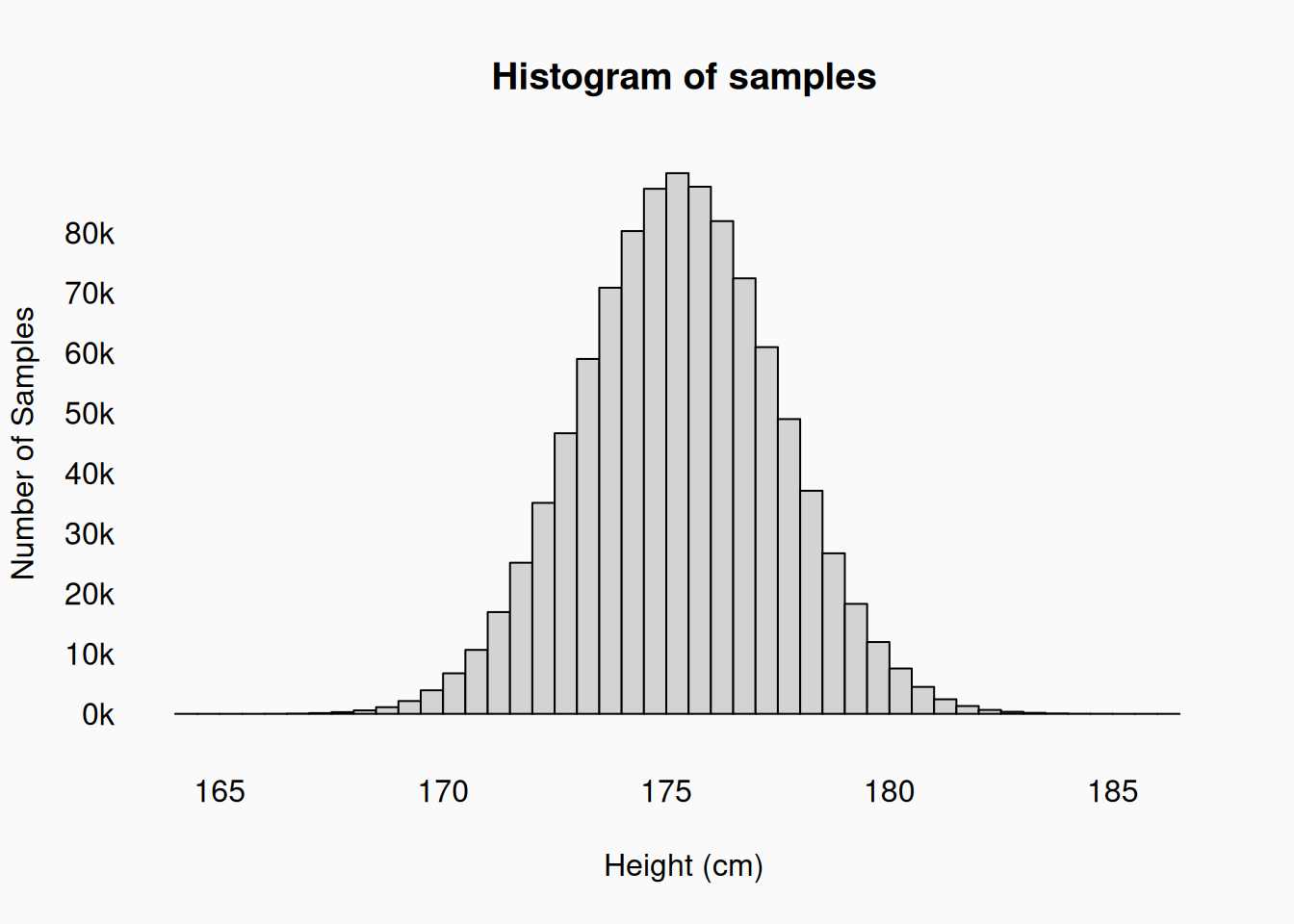
With a million sample means, we can see that the sampling distribution is not just any “bell shape,” but specifically a normal distribution. In fact, one of the fundamental theories of statistics—the central limit theorem—, which tells us that the distribution of sample means (\(\bar{x}\)) is normally distributed, centered at the population mean (\(\mu\)). This is true for samples drawn from any probability distribution! What’s more, the standard deviation of the sample mean distribution will be \(\frac{\sigma}{\sqrt{N}}\), where \(N\) is the size of each sample.2
The “distribution of sample means” is one of the most fundamental concepts in classical statistics. Because it is so important, the standard deviation of the distribution of sample means has its own special name: the standard error. It is often abbreviated things like SE, SEM (standard error of mean), or Std. Error.
Confidence
Now, in the real world we don’t get to take thousands of independent samples from a population. We typically take one. The mean of our one sample will not be the same as the population mean. Even if we sample a thousand people, we will always—simply by chance—have sampled a group of people who are shorter or taller than average, at least by a small amount. And sometimes—rarely—by a large amount. How can we know if our one sample mean is close to the population mean, or way off? We can never know, but we can still make some reasonable inferences.
If we understand the sampling distribution of the statistics we calculate, we can use that knowledge to make precise inferences about just how improbable different errors would be. For example, we can characterize the interquartile range of our sampling distribution. If the population has a mean \(\mu = 175.3_{cm}\) and a standard deviation of \(\sigma = 7_{cm}\), then 50% of the sample means should fall in the range \([173.8_{cm}, 176.8_{cm}]\). In other words, half of our samples (of ten men) should be within \(\approx1.5_{cm}\) of the true (population) mean. This is called the 50% confidence interval. It is very common to report the 95% confidence interval, capturing the middle 95% of the sampling distribution for a statistic; in this case the 95% confidence interval is \([171.0_{cm}, 179.6_{cm}]\). Confidence intervals are often drawn with brackets around sample means on plots.
Assumptions
All analyses are based on assumptions, and statistics are no different. Most fundamentally, we are assuming that our samples are truly random samples from the population we want to make claims about. If for example, we recruited a lot of men hanging out at basketball courts, our sample might be biased towards higher heights. What’s more, our calculation of the standard error assumes that each and every data point is sampled independently; i.e., that the data is not “sticky.” If, for example, some of the men in our sample are siblings, their heights might be correlated. If the data points are correlated, there is less information in the data and the effective sample size is actually smaller than the observed \(N\), which throws off the calculation of the standard error.
Sample Size
The sample size is denoted \(N\). Above, I told you that the sample mean is a consistent statistic, so the larger \(N\) is, the closer our sample means (\(\bar{x}\)) should get to the population mean (\(\mu\)).
\[ \lim_{N\to\infty} |\bar{x} - \mu| \to 0 \]
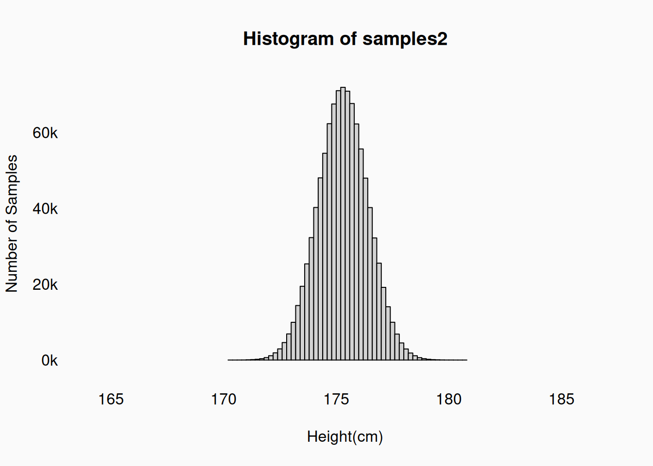
This is a result of the law of large numbers. In fact, the definition of the standard error—\(\frac{\sigma}{\sqrt{N}}\)—tells precisely how much closer we’ll get to the population mean on average. If we increase the size of each of our samples by four fold, the standard error should be cut in half (the square root of four). To check that this is right, let’s take another sample of one million sample means but this time make each sample contain 40 men, instead of 10:
What if we up our sample size to 200 men?
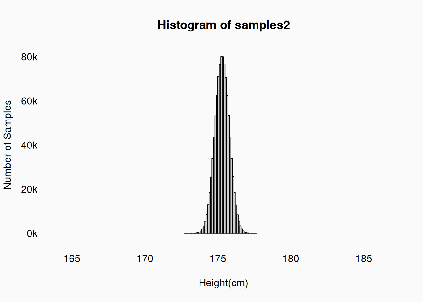
The larger the sample size, the more tightly our consistent statistic clusters around the true population mean. If we understand the sampling distribution of the statistics we calculate, we can use that knowledge to make more precise inferences about the population. With a 200-man sample, half of our samples should be within \(0.33_{cm}\) of the true (population) mean, and even our 95% confidence interval is shrunk to \([174.3_{cm}, 176.3_{cm}]\).
Sample Sizes
So, obviously bigger samples are better, but how big do samples actually need to be? As is often the case, sample size is usually determined by practicality more than anything else. Even if you’d like to recruit 200 participants for a user study, you might only get 10.
Fortunately, if sampling is truly random (and independent), even small samples can lead to surprisingly good estimates, and increasing the sample size beyond a point has quickly diminishing returns. For example, here is a graph of the standard error (in our men-height scenario) as a function of sample size:
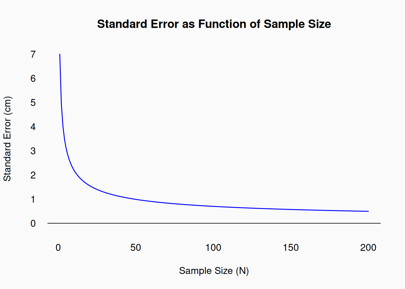
Sampling 25 men is already a huge improvement over 10 men, but boosting it to 100 men is not nearly as much help.
Ultimately, to guess an appropriate sample size we must consider the effect size we expect to see, relative to the amount of error in the data. If all we want to do is demonstrate that men are (on average) taller than women, we might not need a very big sample. Why? Because we can anticipate that the effect of sex on height is probably around \(10_{cm}\) or more. However, if we instead hypothesized that cellists are taller (on average) than violinists, we might expect the effect to be fairly small.3 If cellists were truly only \(\approx1_{cm}\) taller than violinists, we’d need to shrink our confidence intervals down quite a lot in order to make a valid claim about that small effect.
If the effects we are studying are strong, even a small sample size can be sufficient. If the effects we are studying are subtle, or if the data is really noisy, we need more data. Estimating the appropriate sample size for statistical tests is called statistical power—which we will learn about in our chapter on Effect Size.
The Law of Small Numbers
US Counties
There are 3,141 counties in the United States. Some of these counties have higher rates of cancer than others. The lowest cancer rates are evident in sparsely populated rural areas, especially in the West, Midwest, the South, and Alaska. These counties also tend to be politically Republican. Why do you suppose these counties have lower cancer rates?
One possibility is that these counties have less air and water pollution, and that people in rural areas are more likely to engage in regular physical activity. It is also possible that people in rural areas eat a healthier diet with fewer food additives. Another possibility is that strong religious convictions lead to cleaner living with less drug or alcohol abuse. Perhaps the closer friendships and community values found in rural areas tend to lower stress. What do you think? Are these plausible explanations for the lower cancer rates?
We might find it helpful to contrast these counties with those U.S. counties that have the highest rates of cancer. The highest cancer rates are evident in sparsely populated rural areas, especially in the West, Midwest, the South, and Alaska. These counties also tend to be politically Republican.
What’s wrong here?
Let’s consider the implicit null hypothesis for this example.
\(H_0\): the true cancer incidence rate is equal across all US counties.
Suppose that the true cancer rate in the USA is 0.1% of the population per year. Any sample from the US population can be used to estimate that population value;
- If we use small samples, our estimates will be more varied. For example, if we measure the cancer rate of people living in Taliaferro County, Georgia (pop. 1,600), we’d expect to see 0 cancer cases (0% rate) 1 year out of five, and four cases (2.5% rate) one year out of twenty. Thus, if we measured twenty small counties, we’d expect to see four with 0% cancer rates and one with a 2.5% (very high) cancer rate.
- In contrast, if we take larger samples, our estimates of the cancer rate will be more precise. For example, if we measure the cancer rate of people living in Fulton County (pop. 1,074,634), we’d only expect to see a cancer rate below 0.09% every 2,231 years, or above 0.11% every 1,700 years.
So, our observation that the lowest and the highest cancer rates in the USA occur in small counties is consistent with the null hypothesis. The reason that extreme cancer rates (good and bad) show up in small counties is simply because they are smaller samples.
Daniel Kahneman (2012) summarizes the problem in the following way:
You must exert some mental effort to see that the following two statements mean exactly the same thing: - Large samples are more precise than small samples. - Small samples yield extreme results more often than large samples do. The first statement has a clear ring of truth, but until the second version makes intuitive sense, you have not truly understood the first. (Kahneman, 2012; p.111)
Unequal sample sizes
We already knew that bigger samples are better, and smaller samples are worse. These illustrations of the “law of small numbers” teach us another lesson: Be cautious when sample sizes are unequal! If you have a sample of 44 jazz tracks, and 903 hip-hop tracks, the statistical estimates in the jazz subset will be much less precise than in the hip-hop subset.
- An encoding of a classical symphony score might have many thousands of notes in it. A jazz lead sheet might have 100–200 notes in it. Features extracted from the jazz piece will be less certain than those from the classical piece.
- An average pop song from the 1950s is much shorter than one from the 2010s. Again, features extracted from earlier tracks will be more varied than from more recent tracks.
Generally, in research, we aim to sample equally from all experimental conditions. The ideal is a “full factorial” design, where all combinations of our research variables are measured in equal amounts. This is why stratified sampling is such an important technique.
Mantras
Big values are found in small places
The law of large numbers doesn’t apply to small numbers. Smaller subsets will often have the most extreme values. If your data is divided into subsets, the smallest subsets will likely have the most variability and most extreme averages.